Excel Array Formula Examples: 7 Tips to Master Spreadsheets

Unleash the Power of Excel Array Formulas

Excel array formulas offer a powerful way to perform complex calculations and manipulate data efficiently. This listicle provides seven practical examples of Excel array formulas, complete with step-by-step explanations and actionable takeaways. You'll learn how these formulas work and how to apply them to your own projects.

Whether you're a data analyst, financial expert, or simply an Excel enthusiast, these examples will showcase the versatility of array formulas. Discover how to streamline your workflow and gain deeper insights from your data. This listicle covers:

1. SUM with Multiple Criteria Using Array Formulas
2. Dynamic Array UNIQUE Function for Removing Duplicates
3. Matrix Multiplication Using MMULT
4. Frequency Distribution with FREQUENCY Function
5. Transpose and Reshape Data with TRANSPOSE
6. Lookup Arrays with INDEX-MATCH Array Formulas
7. Multi-Criteria Filtering with Dynamic Arrays

We'll analyze each excel array formula example, demonstrating the strategic "why" behind its effectiveness, and provide specific tactical insights for practical application. Learn how combining these formulas unlocks even more powerful solutions, expanding the possibilities within Excel. Prepare to optimize your spreadsheets and unlock the true potential of your data.

1. SUM with Multiple Criteria Using Array Formulas

This powerful technique allows you to sum values based on multiple criteria across different columns or ranges within Excel. It leverages the multiplication of boolean arrays (TRUE/FALSE values) to effectively create logical AND conditions. This provides a robust alternative to the SUMIFS function, particularly when dealing with complex scenarios where SUMIFS might fall short. This method is crucial for anyone working with data analysis in Excel, offering more control and flexibility in calculations. This technique is essential for any Excel user aiming to master advanced formula capabilities.

How It Works

Array formulas in this context treat ranges of cells as arrays of values. When comparing these arrays against criteria, the result is an array of TRUE/FALSE values. Multiplying these boolean arrays effectively performs a logical AND operation: TRUE * TRUE = 1, while any other combination (TRUE * FALSE, FALSE * TRUE, FALSE * FALSE) equals 0. Finally, the SUM function adds up the resulting 1s, which correspond to the values that meet all criteria.

Examples of Successful Implementation

Several situations showcase the effectiveness of this technique:

• Sales Reporting: Sum revenue by region AND product category. This allows for granular analysis of sales performance across different segments.
• Inventory Management: Sum quantities by warehouse AND date range. This provides accurate inventory snapshots for specific periods.
• Financial Analysis: Sum expenses by department AND cost center. This enables detailed cost analysis and budget control.

Actionable Tips and Best Practices

• Named Ranges: Use named ranges to make your formulas more readable and easier to understand. For example, instead of A1:A10, you might use a named range like SalesRegion.
• Start Small: Test your array formulas with small datasets first to ensure they work correctly before applying them to large ranges. This prevents errors and simplifies debugging.
• SUMPRODUCT Alternative: Consider SUMPRODUCT as an alternative to array formulas for multiple criteria sums. SUMPRODUCT performs similarly but doesn't require the special Ctrl + Shift + Enter array entry. Learn more about using SUMPRODUCT for multiple criteria sums here.
• Helper Columns: For exceptionally complex criteria, break them down into separate helper columns. This simplifies the main formula and makes debugging easier.

Visualizing the Process

The following infographic illustrates the step-by-step process of summing with multiple criteria using array formulas. It visualizes how boolean arrays are used to filter and sum values based on defined criteria.

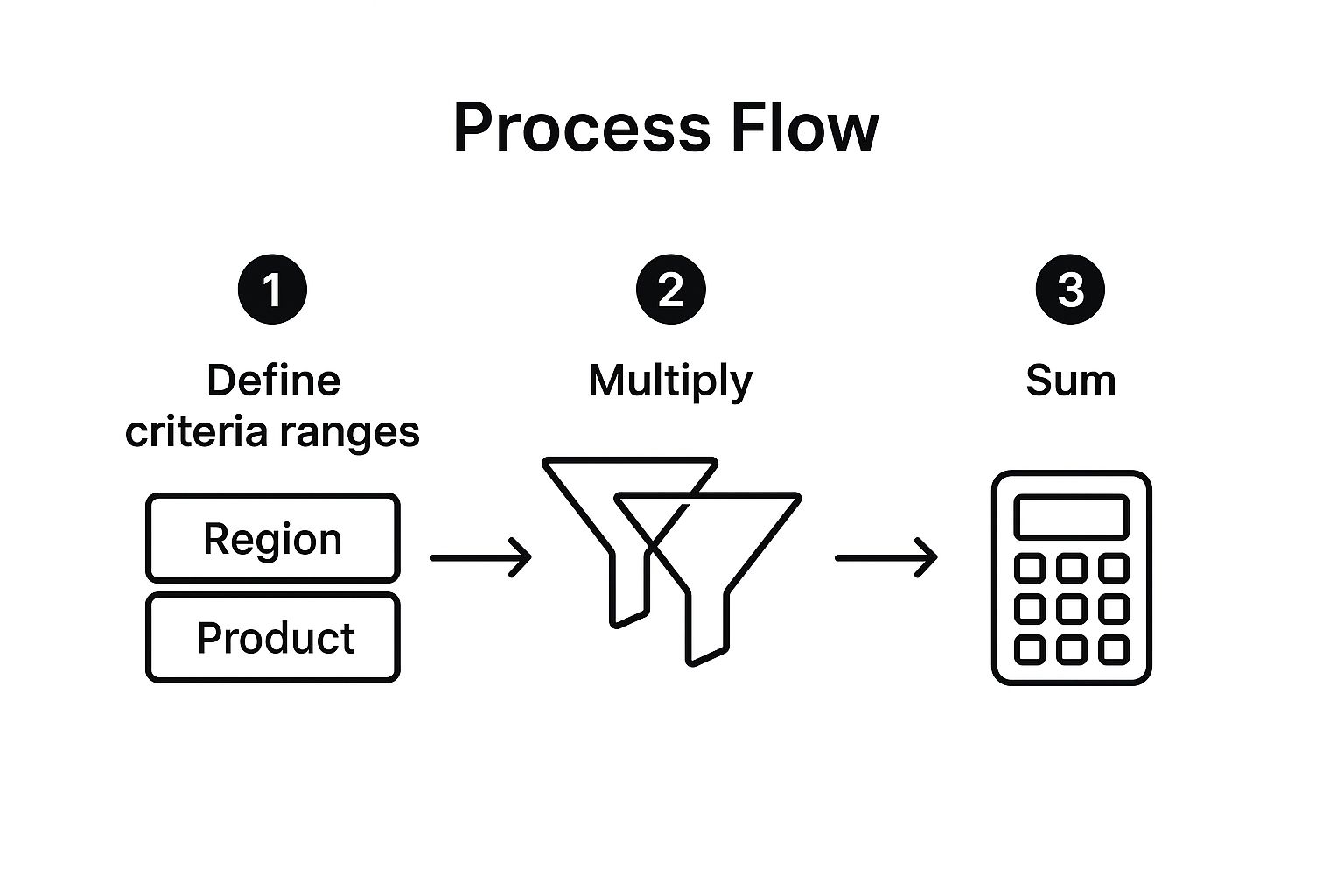
The infographic clearly demonstrates the flow: defining criteria ranges, multiplying boolean arrays for logical AND, and finally summing the filtered values. This visual representation clarifies the logic behind this powerful Excel array formula example.

This method deserves a prominent place in any list of essential Excel array formulas because it offers a flexible and efficient way to handle complex data analysis tasks. Mastering this technique empowers users to extract meaningful insights from their data, streamlining reporting and decision-making processes.

2. Dynamic Array UNIQUE Function for Removing Duplicates

This innovative function, introduced as part of the dynamic array engine in Excel 365 and Excel 2021, streamlines the process of extracting unique values from a dataset. It automatically spills the results into adjacent cells, eliminating the need for manual copying or complex formulas. This dynamic behavior makes UNIQUE a game-changer for data cleaning, list management, and various data analysis tasks within Excel. It signifies a leap forward in efficiency for anyone working with large datasets or needing to quickly isolate unique entries.

How It Works

The UNIQUE function operates on a given range or array, identifying and returning only the distinct values. It intelligently handles both vertical and horizontal ranges, adapting the spill range accordingly. The dynamic nature means the output automatically adjusts if the source data changes, ensuring the unique list stays current. This eliminates the need to constantly update formulas, saving time and reducing the risk of errors.

Examples of Successful Implementation

The UNIQUE function proves invaluable in several scenarios:

• Customer Relationship Management (CRM): Extract a unique list of customer emails from a transaction database for targeted marketing campaigns.
• Inventory Control: Generate a list of unique product SKUs from an inventory spreadsheet for simplified stocktaking and analysis.
• Data Validation: Create dropdown lists with only unique entries from a source range, preventing duplicate data entry.

Actionable Tips and Best Practices

• Spill Range Management: Ensure sufficient blank cells below and to the right of the UNIQUE formula to accommodate the spilled results. Obstructions will cause a #SPILL! error.
• Sorted Unique Values: Use SORT(UNIQUE(range)) to obtain a sorted list of unique values, enhancing readability and further analysis.
• Filtering Unique Values: Combine UNIQUE with FILTER to extract unique values that meet specific criteria, providing even more granular control. Learn more about data scrubbing techniques, including using UNIQUE, at this helpful resource.
• Multi-Column Uniqueness: Leverage the by_col parameter within UNIQUE to determine uniqueness based on specific columns in a multi-column range.

When and Why to Use UNIQUE

The UNIQUE function is particularly beneficial when:

• Dealing with large datasets where manual identification of duplicates is time-consuming and prone to errors.
• Requiring a dynamic list of unique values that automatically updates with changes to the source data.
• Simplifying data cleaning and validation by quickly isolating unique entries and removing redundant information.

This dynamic array formula deserves a place among essential Excel array formula examples due to its ability to streamline data management and analysis. Its automatic spilling behavior, coupled with its flexibility in handling various data scenarios, makes it a powerful tool for any Excel user seeking increased efficiency and accuracy in their work.

3. Matrix Multiplication Using MMULT

This powerful array formula performs matrix multiplication directly within Excel. MMULT is essential for advanced mathematical computations, enabling everything from financial modeling and engineering calculations to data science applications and operations research. This function is a cornerstone for handling complex data interactions and provides a robust alternative to manual matrix multiplication, saving considerable time and reducing the risk of errors. This function is invaluable for any Excel user working with matrices and requiring advanced calculations.

How It Works

MMULT takes two arrays as arguments and returns their matrix product. The crucial requirement is that the number of columns in the first array must equal the number of rows in the second array. The resulting matrix will have the same number of rows as the first array and the same number of columns as the second. The calculation itself involves multiplying corresponding elements of the rows of the first matrix by the columns of the second and then summing the products.

Examples of Successful Implementation

The versatility of MMULT is showcased in its diverse applications:

• Financial Modeling: Calculate portfolio risk by multiplying a portfolio weights matrix by a covariance matrix. This allows for rapid risk assessment and informed investment decisions.
• Engineering: Perform structural analysis by multiplying a stiffness matrix by a displacement vector to determine forces and stresses in a structure. This simplifies complex engineering calculations within Excel.
• Data Science: Conduct dimensionality reduction using techniques like Principal Component Analysis (PCA) which relies heavily on matrix operations including MMULT. This simplifies datasets while preserving critical information.

Actionable Tips and Best Practices

• Dimension Check: Always double-check that the number of columns in the first array matches the number of rows in the second. This prevents common #VALUE! errors.
• Named Ranges: Enhance formula readability by using named ranges for the matrices. This makes the formula easier to understand and reduces the chance of referencing incorrect cells.
• Performance Considerations: For extremely large matrices, break the calculation down into smaller, manageable chunks. This can improve performance and prevent potential crashes.
• Transpose Integration: Combine MMULT with the TRANSPOSE function to perform more advanced matrix manipulations. This opens up a wide range of possibilities for complex calculations.

This array formula deserves its place in any list of essential Excel array formula examples because it provides a direct and efficient method for matrix multiplication. This eliminates the need for tedious manual calculations, allowing users to focus on interpreting the results rather than getting bogged down in the process. Mastering MMULT empowers Excel users to leverage the power of linear algebra for advanced analysis and modeling across a wide range of disciplines.

4. Frequency Distribution with FREQUENCY Function

This essential technique allows you to create frequency distributions by counting how many values fall within specified intervals, often referred to as "bins." The FREQUENCY function is a powerful tool for statistical analysis, data visualization preparation, and understanding the distribution of your data within Excel. This function is crucial for anyone working with data analysis, providing a clear picture of data distribution. Mastering this technique elevates any Excel user's analytical capabilities.

How It Works

The FREQUENCY function takes two arguments: the data_array (the range of values you want to analyze) and the bins_array (the boundaries of your intervals). It returns an array of frequencies, where each element represents the count of values within a corresponding bin. This function is an array formula, meaning it returns multiple values simultaneously and must be entered using Ctrl + Shift + Enter.

Examples of Successful Implementation

The FREQUENCY function proves invaluable in various scenarios:

• Sales Analysis: Determine the distribution of order values across different price ranges. This helps understand customer purchasing behavior and identify popular price points.
• Quality Control: Analyze the distribution of measurement values across tolerance bands. This allows for identification of deviations from expected standards and improved quality control processes.
• Survey Research: Create age group distributions from demographic studies. This helps understand the age demographics of respondents and tailor future surveys accordingly.
• Performance Metrics: Analyze response time distributions in service analysis. This identifies areas where service delivery is slow and allows for optimization.

Actionable Tips and Best Practices

• Define Bins Carefully: Ensure your bin ranges are defined logically to avoid gaps or overlaps. Accurate bins are essential for generating meaningful frequency distributions.
• Histogram Creation: Use the output of the FREQUENCY function to create histograms. Visualizing the distribution enhances understanding and communication of insights.
• Analysis ToolPak: Explore the Analysis ToolPak for additional statistical analysis functions. This add-in extends Excel's statistical capabilities for advanced users.
• Dynamic Bin Labeling: Combine FREQUENCY with MATCH and INDEX for dynamic bin labeling. This allows for automatic adjustment of labels as bin ranges change.

This method earns its place among essential Excel array formulas because it provides a fundamental method for analyzing data distributions. Understanding how your data is distributed is key to making informed decisions and extracting valuable insights. The FREQUENCY function empowers users to visualize patterns and trends within their data, enhancing reporting and analysis processes.

5. Transpose and Reshape Data with TRANSPOSE

This essential array formula, TRANSPOSE, dynamically flips the orientation of your data, converting rows into columns and columns into rows. This is invaluable for restructuring data, making it compatible with different reporting formats, or preparing datasets for specific types of analysis. TRANSPOSE provides a powerful solution for data manipulation within Excel, enabling users to adapt and utilize information effectively. This flexibility is critical for anyone working with data in Excel, from simple reports to complex analytical models.

How It Works

TRANSPOSE takes a range of cells as input and outputs a transposed version of that range. The number of rows in the input becomes the number of columns in the output, and vice versa. This dynamic restructuring allows for quick and efficient data reformatting without manual data entry or complex manipulations. The array formula nature of TRANSPOSE means it works with entire ranges of data at once, simplifying data transformation tasks.

Examples of Successful Implementation

• Report Formatting: Convert monthly sales data from rows (each month a row) to columns (each month a column) for a clear dashboard visualization.
• Data Import: Restructure imported data from a database or CSV file to match your existing Excel templates and reporting layouts.
• Survey Analysis: Transpose respondent answers from a horizontal format (one respondent per row) to a vertical layout (one question per row) for easier analysis and charting.
• Financial Reporting: Transform quarterly financial data orientation to accommodate different stakeholder requirements or reporting standards.

Actionable Tips and Best Practices

• Sufficient Space: Ensure the target range for the transposed data has enough empty cells to accommodate the new dimensions. TRANSPOSE will overwrite existing data.
• Dynamic Arrays (Excel 365): In Excel 365, TRANSPOSE benefits from dynamic arrays, automatically updating the transposed data when the source data changes.
• Paste Special: For a quick, one-time transposition, consider using the "Paste Special" > "Transpose" option. This is a simpler alternative for static data transformations.
• Combining with Other Functions: Combine TRANSPOSE with other functions like INDEX to perform selective transposition of specific rows or columns.
• Power Query for Complex Transformations: For even more advanced data transformation needs, consider using Power Query. Learn more about using Power Query for data transformation.

When and Why to Use This Approach

Use TRANSPOSE when you need to change the orientation of your data, specifically rows to columns or vice versa. This is particularly useful when:

• Data from external sources doesn't align with your reporting needs.
• You need to prepare data for certain types of analysis or charting.
• Creating dynamic dashboards that respond to changes in source data.

This function is a cornerstone of efficient data manipulation in Excel. Its dynamic nature and ability to restructure entire data ranges with a simple formula make it an essential tool for any Excel user working with data. Mastering TRANSPOSE unlocks significant potential for data analysis, reporting, and overall spreadsheet efficiency.

6. Lookup Arrays with INDEX-MATCH Array Formulas

This powerful technique combines the INDEX and MATCH functions within an array formula to create a highly flexible and efficient lookup solution in Excel. It surpasses the limitations of traditional VLOOKUP by enabling searches in any direction (not just left-to-right) and accommodating multiple criteria. This method is especially valuable for complex data retrieval scenarios where VLOOKUP falls short, and it's a must-have skill for anyone working with large datasets or intricate lookup requirements in Excel. Mastering this approach provides significant advantages in data analysis and reporting.

How It Works

The INDEX function retrieves a value from a specified range based on its row and column number. MATCH finds the position of a value within a range. When combined within an array formula, MATCH can return an array of positions, and INDEX uses this array to retrieve multiple values simultaneously. This synergy allows for lookups based on complex criteria combinations, enabling sophisticated data extraction.

Examples of Successful Implementation

Several scenarios demonstrate the effectiveness of INDEX-MATCH array formulas:

• Employee Database: Find employee details (name, salary, department) based on multiple criteria, such as department and position. This allows for precise filtering and reporting within HR datasets.
• Inventory Management: Lookup product information (price, stock level, supplier) using a combination of identifiers like product code and color. This improves inventory tracking and analysis.
• Financial Reporting: Retrieve account balances based on account code and reporting period. This facilitates efficient financial analysis and reporting.
• Sales Analysis: Find sales data for specific products within a certain region and time period, allowing for detailed analysis of sales performance.

Actionable Tips and Best Practices

• Named Ranges: Use named ranges to improve formula readability and maintainability. For example, name your employee data range EmployeeData instead of referring to it as A1:F100.
• Test Components Separately: Test your INDEX and MATCH formulas individually before combining them into an array formula. This helps isolate and resolve any errors quickly.
• XLOOKUP Consideration: If you're using a newer version of Excel, consider XLOOKUP as a potentially simpler alternative for complex lookups.
• Error Handling: Use IFERROR to handle cases where a match isn't found. This prevents errors from disrupting your spreadsheet and provides a cleaner output. Learn more about comparing INDEX-MATCH vs. VLOOKUP at this link.

This technique is a crucial addition to any list of essential Excel array formula examples due to its versatility and power. By mastering INDEX-MATCH array formulas, users can overcome the limitations of traditional lookup methods, enabling more complex data retrieval and analysis for enhanced reporting and decision-making.

7. Multi-Criteria Filtering with Dynamic Arrays

This method revolutionizes data filtering in Excel. The FILTER function dynamically returns filtered results based on multiple criteria, creating live, updating datasets without the limitations of traditional AutoFilter. This dynamic approach is crucial for interactive dashboards and reports where real-time data manipulation is essential. It's a game-changer for anyone working with large datasets and complex filtering requirements.

How It Works

FILTER takes an array as input and returns a subset based on specified criteria. Multiple criteria can be combined using boolean logic (AND/OR) to create complex filters. Unlike static filtering methods, FILTER produces a dynamic array that updates automatically when the source data or criteria change. This provides unparalleled flexibility for interactive analysis.

Examples of Successful Implementation

Several applications showcase the power of dynamic array filtering:

• Sales Reporting: Filter transactions by date range, salesperson, and product category to analyze specific sales trends. This allows for granular insights into sales performance.
• Project Management: Display tasks assigned to specific team members with certain statuses to track project progress effectively. This fosters clear visibility into team workloads and project timelines.
• Inventory Analysis: Show products below reorder levels in specific categories to prioritize restocking efforts. This improves inventory control and prevents stockouts.
• Customer Analysis: Filter customers by purchase history and geographic location for targeted marketing campaigns. This enables personalized customer engagement and improved marketing ROI.

Actionable Tips and Best Practices

• Parentheses for Logic: Use parentheses to control the order of operations when combining AND/OR logic within your filter criteria. This ensures accurate filtering based on intended logic.
• Sorting with SORT: Combine FILTER with the SORT function to create dynamically sorted and filtered views. This improves data presentation and facilitates easier analysis.
• Counting with COUNTA: Use COUNTA on the filtered results to dynamically count the number of items that meet the criteria. This provides a live count that updates with the filtered data.
• Nested FILTER Functions: For complex multi-stage filtering, nest FILTER functions to apply successive filters on the results of previous filters. This allows for granular filtering of data based on multiple levels of criteria.

When and Why to Use This Approach

Use FILTER when you need interactive, dynamic filtering capabilities beyond what traditional AutoFilter offers. It's ideal for situations where the criteria or data might change frequently and you require real-time updates to your filtered results. Learn more about Multi-Criteria Filtering with Dynamic Arrays techniques and similar approaches to advanced filtering in Excel here. This approach is particularly effective for creating dashboards and reports that require user interaction and data exploration.

This method is a must-have in any list of excel array formula examples because it represents a significant advancement in data manipulation capabilities. It empowers users to create truly interactive reports and dashboards, significantly improving data analysis workflows. This dynamic filtering capability is a major advantage for anyone working with data in Excel.

7 Key Excel Array Formula Examples Comparison

Technique	Implementation Complexity 🔄	Resource Requirements ⚡	Expected Outcomes 📊	Ideal Use Cases 💡	Key Advantages ⭐
SUM with Multiple Criteria Using Array Formulas	Intermediate	Moderate to High (memory intensive with large data)	Accurate summation based on multiple conditions	Sales reporting, inventory management, financial analysis	More flexible than SUMIFS, handles complex conditions
Dynamic Array UNIQUE Function for Removing Duplicates	Beginner	Low	Clean, unique lists that update dynamically	Data cleaning, list management, survey analysis	Simple syntax, automatic updates, removes duplicates
Matrix Multiplication Using MMULT	Advanced	High (computationally intensive for large matrices)	Precise matrix multiplication results	Financial modeling, engineering, data science	Enables sophisticated math modeling with accuracy
Frequency Distribution with FREQUENCY	Intermediate	Moderate	Frequency counts for specified bins	Statistical analysis, quality control, survey research	Fast statistical summaries, foundation for histograms
Transpose and Reshape Data with TRANSPOSE	Beginner	Low	Data orientation flipped (rows ↔ columns)	Report formatting, data import, survey analysis	Essential for data restructuring, maintains integrity
Lookup Arrays with INDEX-MATCH Array Formulas	Intermediate	Moderate	Flexible, multi-criteria lookups	Databases, report generation, data validation	More powerful than VLOOKUP, supports multi-directional searches
Multi-Criteria Filtering with Dynamic Arrays	Intermediate	Moderate	Live filtered datasets with multiple criteria	Sales reporting, project management, inventory analysis	Dynamic, no helper columns needed, integrates with other functions

Level Up Your Spreadsheet Game with SumproductAddict

This journey through the world of Excel array formula examples has demonstrated their immense power and versatility. From simplifying complex calculations like multi-criteria sums and dynamic lookups to manipulating data with matrix multiplication and transposition, array formulas offer elegant solutions to everyday spreadsheet challenges. By understanding the core principles behind these examples, you can adapt and apply them to a wide range of scenarios, transforming your workflows and boosting your analytical capabilities.

Key Takeaways and Actionable Insights

Let's recap some of the most important takeaways from the examples we've covered:

• Efficiency: Array formulas consolidate multiple operations into a single formula, reducing clutter and improving spreadsheet performance. This is especially noticeable when working with large datasets.
• Flexibility: Whether you're dealing with dynamic arrays, unique value extraction, or multi-criteria filtering, array formulas offer the flexibility to tackle diverse data manipulation tasks.
• Data Integrity: By performing calculations in memory and returning results directly to the spreadsheet, array formulas minimize manual data entry, thus reducing the risk of errors.

Why Master Excel Array Formulas?

Mastering Excel array formulas is more than just adding another tool to your spreadsheet arsenal. It’s about transforming your approach to data analysis. By understanding how to leverage the power of array formulas, you can:

• Automate complex tasks: Spend less time on tedious manual calculations and more time on interpreting your results.
• Improve data accuracy: Reduce errors and ensure data integrity by minimizing manual data entry.
• Gain deeper insights: Unlock the full potential of your data and uncover hidden trends.

From Formulas to Fashion: Embrace Your Inner Excel Pro

These examples have shown you how to wield the power of "excel array formula examples" like a pro. But why stop there? Take your spreadsheet enthusiasm to the next level with SumproductAddict. We offer a unique collection of Excel-themed apparel and accessories, perfect for showcasing your love for spreadsheets.

Next Steps: Practice and Explore

The key to mastering array formulas is practice. Experiment with the examples provided, adapt them to your own spreadsheets, and explore the vast resources available online. As you become more comfortable with array formulas, you’ll discover even more creative and powerful ways to use them.

Want to celebrate your newfound Excel mastery? Visit SumproductAddict and use code EXCELPRO for a discount on your first order. Show your spreadsheet pride with our unique designs!