Excel Formula Cheat Sheet: Master 7 Essential Formulas

Unlocking Excel's Power with Essential Formulas

This Excel formula cheat sheet equips you with seven essential formulas to conquer any spreadsheet challenge. Learn how to efficiently search data with VLOOKUP, INDEX/MATCH, and XLOOKUP. Master conditional summing and counting with SUMIF/SUMIFS and COUNTIF/COUNTIFS. Control data flow with IF/IFS statements. Finally, combine and format text like a pro using CONCATENATE/TEXTJOIN. These formulas are crucial for data analysis and reporting, boosting your productivity whether you're an Excel novice or a spreadsheet guru.

1. VLOOKUP

VLOOKUP (Vertical Lookup) is a cornerstone function in Excel's formula repertoire, earning its place in any "excel formula cheat sheet" due to its widespread use and power in retrieving data from tables. It's a go-to tool for anyone working with structured data, from data analysts to accountants, making it an essential skill for efficient spreadsheet management. This function searches for a specific value in the first column of a given table and returns a corresponding value from a designated column in the same row. Its simple syntax and powerful functionality make it a must-have in any Excel user's toolkit.

The syntax of VLOOKUP is: =VLOOKUP(lookup_value, table_array, col_index_num, [range_lookup])

Let's break down each part:

• lookup_value: The value you're searching for in the first column of the table. This can be a number, text, or a cell reference containing the value.
• table_array: The range of cells that contains your data table, including the lookup column and the column containing the value you want to return. Crucially, the lookup column must be the leftmost column in this range.
• col_index_num: The column number within the table_array from which you want to retrieve the corresponding value. The leftmost column in table_array is considered column 1.
• [range_lookup]: This optional argument specifies whether you want an exact or approximate match. Use FALSE for an exact match and TRUE for an approximate match (requires sorted data). If omitted, the default is TRUE.

VLOOKUP is particularly useful when dealing with structured datasets resembling databases. Consider these examples:

• Employee Databases: Find an employee's salary by looking up their employee ID.
• Product Catalogs: Determine the price of a product by searching for its product code.
• Student Records: Retrieve a student's grade by looking up their student number.
• Inventory Management: Get the stock level of an item by searching for its SKU.

Features and Benefits:

• Searches Vertically: Efficiently searches down the first column of your specified range.
• Returns Values from Columns to the Right: Retrieves data from any column to the right of the lookup column.
• Exact or Approximate Matching: Offers flexibility for different lookup needs.
• Case-Insensitive: Simplifies lookups without worrying about case sensitivity.
• Industry Standard: Widely understood and used, making collaboration easier.

Pros:

• Wide Compatibility: Works across all Excel versions.
• Intuitive: Relatively easy to learn and use.
• Efficient for Structured Data: Excels with well-organized tables.
• Fast Processing (Moderate Datasets): Performs well with datasets of reasonable size.

Cons:

• Leftward Lookup Limitation: Cannot search to the left of the lookup column.
• Column Insertion/Deletion Issues: Formulas can break if columns are inserted or deleted within the table_array.
• Returns Only First Match: If multiple matches exist, only the first one is returned.
• Performance Degradation (Large Datasets): Can become slow with very large datasets.
• Approximate Match Requires Sorted Data: For approximate matches, the lookup column must be sorted in ascending order.

Tips for Effective VLOOKUP Usage:

• Exact Matches: Always use FALSE for range_lookup unless you specifically require an approximate match.
• Absolute References: Use absolute references (e.g., $A$1:$C$10) for the table_array when copying formulas to prevent unintended range shifts.
• Alternatives for More Flexibility: Consider using INDEX/MATCH or XLOOKUP for more complex lookups, especially when needing to search to the left or requiring more dynamic functionality.
• Sort Data for Approximate Matches: If using TRUE for range_lookup, ensure your lookup column is sorted in ascending order.
• Error Handling: Implement error handling with IFERROR to manage #N/A errors and provide alternative outputs.

The following infographic provides a simple decision tree to guide you in choosing the appropriate lookup function and range_lookup setting for your needs:

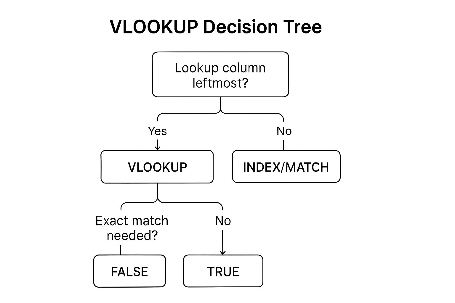
This infographic visualizes the decision process for selecting between VLOOKUP and INDEX/MATCH, and whether to use an exact or approximate match. The key takeaway is that if your lookup column is the leftmost column and you need an exact match, VLOOKUP with FALSE is the way to go. Otherwise, consider INDEX/MATCH or ensure your data is sorted for an approximate match with VLOOKUP using TRUE. By carefully considering these factors, you can leverage the power of lookup functions effectively within your spreadsheets.

2. INDEX/MATCH

The INDEX/MATCH combination is a powerful tool in any Excel user's arsenal, earning its spot on this Excel formula cheat sheet for its versatility and efficiency, especially when dealing with complex lookups. While VLOOKUP is often the go-to for simple lookups, INDEX/MATCH surpasses it in flexibility and performance, making it a favorite among data analysts, financial modelers, and spreadsheet enthusiasts. This dynamic duo allows you to perform lookups in any direction and handle multiple criteria, providing a robust solution for even the most challenging data retrieval tasks.

So, how does this power couple work? INDEX and MATCH are two separate functions that, when combined, create a highly effective lookup formula. The INDEX function retrieves a value from a specified range based on its row and column number. Think of it like picking a specific book from a library shelf. You tell INDEX the shelf (the range) and the position of the book (row and column), and it returns the title. The MATCH function, on the other hand, finds the position of a specific value within a range. It's like asking the librarian where a particular book is located. You provide the book title, and MATCH tells you its position on the shelf.

The magic happens when you combine these two. You use MATCH to find the position of your lookup value in a specific column (the lookup column). Then, you feed that position to INDEX as the row number, specifying the column from which you want to retrieve the corresponding value (the return column). The general formula looks like this: =INDEX(return_column, MATCH(lookup_value, lookup_column, 0)). The 0 in the MATCH function ensures an exact match.

Let's illustrate with a practical example. Imagine you have a table of employee data, including names, departments, and salaries. You want to find the salary of a specific employee, say "John Smith." Your lookup_value is "John Smith," your lookup_column is the column containing employee names, and your return_column is the salary column. The MATCH function finds John Smith's position in the name column, and INDEX uses that position to retrieve his salary from the salary column.

Here are some examples of how INDEX/MATCH can be successfully implemented across various fields:

• Financial Modeling: Looking up historical stock prices from dynamic tables where columns might be added or removed frequently.
• HR Systems: Cross-referencing employee data based on multiple criteria, such as department and job title, to find specific performance reviews.
• Sales Analysis: Finding sales figures for a particular region and product during a specific time period.
• Manufacturing: Matching part specifications across different databases, even if the databases have different structures.

Pros of using INDEX/MATCH:

• Superior Flexibility: Lookups can be performed left, right, up, or down, unlike VLOOKUP which is limited to looking to the right.
• Better Performance: Especially noticeable on large datasets, INDEX/MATCH is generally faster than VLOOKUP.
• Resistant to Structural Changes: Inserting or deleting columns doesn't break the formula, a common issue with VLOOKUP.
• Returns Values from Any Column: You can retrieve data from any column in the table, regardless of its position relative to the lookup column.
• Enables Complex Multi-Criteria Lookups: By using array formulas, you can incorporate multiple lookup criteria.

Cons of using INDEX/MATCH:

• More Complex Syntax: The nested nature of the formula can be intimidating for beginners.
• Requires Understanding of Two Functions: You need to grasp how both INDEX and MATCH work individually.
• Longer Formula Length: Compared to VLOOKUP, the formula is typically longer.
• Less Intuitive for Simple Lookups: For very basic lookups, VLOOKUP might be simpler to implement.

Tips for using INDEX/MATCH effectively:

• Exact Matches: Use 0 as the third argument in MATCH for exact matches.
• Error Handling: Combine with IFERROR to handle situations where the lookup value isn't found.
• Readability: Use named ranges to make your formulas easier to understand and maintain.
• Testing: Start with small datasets to test your formula before applying it to large tables.
• Array Formulas: In older Excel versions, press Ctrl + Shift + Enter to enter array formulas for multi-criteria lookups.

INDEX/MATCH is a valuable tool in the Excel formula cheat sheet, providing significant advantages over traditional lookup methods like VLOOKUP. Its flexibility, performance, and ability to handle complex scenarios make it a must-have skill for anyone working with data in Excel.

3. SUMIF/SUMIFS

Among the essential functions in any Excel formula cheat sheet are SUMIF and SUMIFS. These conditional sum functions empower you to add values within a range based on specified criteria. This makes them incredibly powerful tools for data analysis, reporting, and various other tasks where you need to extract insights from specific subsets of your data. While SUMIF handles situations involving a single criterion, SUMIFS extends this functionality to accommodate multiple criteria. Mastering these functions is a crucial step towards becoming proficient in Excel.

SUMIF uses the following syntax: =SUMIF(range, criteria, sum_range). Here, range represents the range of cells you're evaluating against your criteria, criteria is the condition that must be met, and sum_range contains the values to be summed if the corresponding cell in the range meets the criteria. For example, to sum all sales figures greater than $1000, you could use =SUMIF(Sales,">1000"), where "Sales" is a named range containing the sales data.

SUMIFS, designed for scenarios involving multiple criteria, employs a slightly different syntax: =SUMIFS(sum_range, criteria_range1, criteria1, criteria_range2, criteria2, ...). In this case, sum_range is the range containing the values to sum, followed by pairs of criteria_range and criteria. This structure allows you to specify up to 127 conditions. For instance, to calculate the total sales of "Product A" in "Region East," you would use =SUMIFS(Sales,ProductName,"Product A",Region,"Region East"), assuming "ProductName" and "Region" are named ranges containing respective data.

Features and Benefits:

• Single and Multiple Condition Summation: SUMIF efficiently handles single conditions, while SUMIFS extends this to multiple criteria, providing remarkable flexibility. This allows you to analyze your data based on complex criteria sets.
• Diverse Criteria Support: Both functions work with text, numerical, and date criteria, enabling you to analyze virtually any data type within your spreadsheets.
• Wildcard Usage: Partial text matching is facilitated by the use of wildcards (* and ?), allowing you to sum values even when the criteria aren't exact matches.
• Comparison Operators: You can use comparison operators (>, <, >=, <=, <>) to define criteria based on numerical relationships, adding another layer of flexibility.
• Efficient Handling of Large Datasets: SUMIF and SUMIFS are generally faster than equivalent array formulas, making them suitable for even large datasets. This speed and efficiency are crucial for data analysts and finance professionals working with extensive datasets.
• Wide Compatibility: These functions are compatible across various Excel versions, ensuring consistent performance regardless of your software version.

Pros:

• Essential for conditional data analysis, allowing you to dissect data based on specific parameters.
• Faster than array formulas for similar tasks, ensuring quicker calculations and improved productivity.
• Intuitive syntax makes them accessible to a broad range of users, regardless of their technical expertise.
• Handles large datasets efficiently, allowing for analysis of extensive data volumes.

Cons:

• Summing based on multiple criteria within the same column can be challenging.
• Limited to basic logical operators, making complex AND/OR combinations difficult.
• Criteria must be exact matches unless wildcards are used, potentially requiring extra steps for partial matches.
• Performance can degrade with extremely large ranges.

Examples:

• Sales Reporting: Sum revenue by product category, sales representative, or both.
• Budget Analysis: Calculate total expenses by department, month, or a combination thereof.
• Inventory Management: Sum quantities by location, product type, or both.
• Customer Analysis: Calculate total purchases by region, customer segment, or a combination thereof.

Tips for Effective Usage:

• Enclose text criteria and comparison operators in quotes.
• Utilize cell references for dynamic criteria, making your formulas adaptable to changes in your data.
• Combine with date functions for time-based analysis, enabling analysis within specific timeframes.
• Leverage wildcards (*) for partial text matching, providing flexibility in your criteria.
• For more complex multi-criteria scenarios, consider using SUMPRODUCT. You can learn more about SUMIF/SUMIFS and how they relate to the powerful SUMPRODUCT function.

SUMIF and SUMIFS are indispensable tools in the Excel arsenal, enabling you to perform complex data analysis and reporting tasks efficiently. Their inclusion in any Excel formula cheat sheet is undoubtedly justified, given their versatility and ease of use. By understanding their features, benefits, and limitations, and by applying the tips provided, you can significantly enhance your data analysis capabilities and extract valuable insights from your spreadsheets. They truly are essential functions for anyone from spreadsheet enthusiasts to data analysts and finance professionals.

4. COUNTIF/COUNTIFS: Your Go-To Excel Formula Cheat Sheet Essential

COUNTIF and COUNTIFS are indispensable functions in any Excel user's toolkit, earning their place on this cheat sheet for their power and versatility in conditional counting. Whether you're a data analyst, accountant, or simply someone who works with spreadsheets, understanding these functions will significantly enhance your data analysis capabilities. They offer a simple yet powerful way to analyze and interpret your data by counting cells that meet specific criteria. This allows you to gain valuable insights and make more informed decisions based on the patterns and trends revealed by your data. This makes them essential additions to any excel formula cheat sheet.

How They Work:

At their core, both functions count cells based on criteria. The key difference lies in the number of criteria they can handle:

• COUNTIF: Designed for single-condition counting. You specify a range and a single criterion, and the function counts the cells within that range that meet the criterion. The syntax is =COUNTIF(range, criteria).

• COUNTIFS: Extends the functionality of COUNTIF to handle multiple criteria. You provide pairs of criteria ranges and criteria, and the function counts only the cells that satisfy all the specified conditions. The syntax is =COUNTIFS(criteria_range1, criteria1, criteria_range2, criteria2, ...).

Features and Benefits:

• Single/Multiple Condition Counting: COUNTIF simplifies single-condition counting, while COUNTIFS handles the complexity of multiple criteria seamlessly.
• Versatile Data Type Support: Both functions work with various data types, including text, numbers, dates, and logical values (TRUE/FALSE).
• Wildcard Support: Use wildcards like "*" (matches any sequence of characters) and "?" (matches any single character) for partial text matches. This is incredibly useful when searching for text strings that contain a certain keyword, but might have variations in the prefix or suffix.
• Comparison Operators: Employ comparison operators (>, <, >=, <=, <>) for numerical range-based counting, allowing for a granular analysis of numerical data.
• Fast Performance: Even with large datasets, these functions perform efficiently, ensuring quick results for your analysis.
• Dashboard and KPI Creation: COUNTIF/COUNTIFS are invaluable for creating interactive dashboards and Key Performance Indicators (KPIs) that update dynamically based on changing data.

Illustrative Examples:

Let's see how these functions work in practice across various fields:

• Quality Control: A manufacturing company can use =COUNTIFS(Date_Range, ">"&DATE(2024,1,1), Shift_Range, "A", Defect_Range, "Yes") to count defective products manufactured after January 1, 2024, during the "A" shift.
• HR Analytics: An HR department can utilize =COUNTIFS(Department_Range, "Marketing", Experience_Range, ">="&5) to count employees in the Marketing department with 5 or more years of experience.
• Customer Service: A customer service team can track ticket counts by priority and status using =COUNTIFS(Priority_Range, "High", Status_Range, "Open").
• Marketing: Marketing teams can count leads by source and conversion status using =COUNTIFS(Source_Range, "Social Media", Conversion_Range, "Converted").

Actionable Tips for Success:

• Counting Non-Specific Values: Use "<>" (not equal to) to count non-blank cells or cells that don't contain a specific value. For example, =COUNTIF(A:A,"<>"") counts all non-blank cells in column A.
• Dynamic Date-Based Counting: Incorporate the TODAY() function for dynamic date-based counting, enabling your spreadsheets to update automatically with current data. =COUNTIF(Date_Range, "<"&TODAY()) counts entries with dates before today.
• Wildcard Text Matching: Leverage the "*" wildcard to count cells containing specific text strings, regardless of their position within the cell. =COUNTIF(Product_Range, "*Apple*") counts all products with "Apple" in their name.
• Dynamic Criteria Referencing: Instead of hard-coding criteria, reference cells containing the criteria. This allows you to easily change the criteria without modifying the formula itself, promoting flexibility and reusability.
• Unique Counting with SUMPRODUCT: For scenarios requiring unique counts, consider combining COUNTIF with the SUMPRODUCT function. Although this is a more advanced technique, it provides a workaround for the lack of built-in distinct count functionality within COUNTIF/COUNTIFS. You can Learn more about COUNTIF/COUNTIFS and explore resources on how to combine these functions effectively.

Pros and Cons:

Pros: Essential for data analysis and reporting, fast performance, simple syntax for complex counting, excellent for dashboards and KPIs, handles various data types.

Cons: Cannot count unique values directly (requires workarounds), limited to basic logical combinations, criteria sensitivity to data formatting.

By mastering COUNTIF and COUNTIFS, you’ll have two powerful tools at your disposal for quickly analyzing and summarizing your data, ultimately unlocking valuable insights and improving your decision-making process. These functions are a must-have in any excel formula cheat sheet.

5. IF/IFS: Mastering Conditional Logic in Your Excel Formula Cheat Sheet

The IF and IFS functions are cornerstones of any comprehensive Excel formula cheat sheet, offering powerful tools for implementing conditional logic within your spreadsheets. They empower you to create dynamic and responsive workbooks that automatically adapt to changing data, making them invaluable for data analysts, business intelligence professionals, accountants, and anyone working with complex datasets. Whether you're calculating commissions, managing projects, or tracking inventory, understanding these functions is essential for maximizing your Excel proficiency.

The IF function allows you to test a single condition and perform different actions based on whether that condition is true or false. Its syntax is straightforward: =IF(logical_test, value_if_true, value_if_false). The logical_test can be any expression that evaluates to TRUE or FALSE. For example, =IF(A1>10, "Greater than 10", "Less than or equal to 10") will display "Greater than 10" if the value in cell A1 is greater than 10 and "Less than or equal to 10" otherwise. This simple structure allows for basic decision-making within your spreadsheets.

The IFS function, introduced in Excel 2016, builds upon the IF function by allowing you to test multiple conditions sequentially. This eliminates the need for complex nested IF statements, which can quickly become unwieldy and difficult to debug. The syntax is =IFS(logical_test1, value_if_true1, logical_test2, value_if_true2, ...). Excel evaluates each logical_test in order, and when it finds a true condition, it returns the corresponding value_if_true. This makes complex conditional logic much more manageable.

Features and Benefits:

• Single vs. Multiple Conditions: IF handles single conditional logic efficiently, while IFS manages multiple conditions without nesting, enhancing readability and maintainability.
• Logical Operators: Both functions support logical operators like AND, OR, and NOT, allowing you to build more complex conditions. For example, =IF(AND(A1>10, B1<20), "Within Range", "Out of Range").
• Versatile Return Values: They can return text, numbers, or even other formulas, providing flexibility in how you use them.
• Automated Decision-Making: These functions are the foundation for automated decision-making in Excel, allowing your spreadsheets to dynamically adapt to changing data.

Illustrative Examples:

• Grade Calculation: Assign letter grades based on numerical scores using IFS: =IFS(A1>=90,"A",A1>=80,"B",A1>=70,"C",A1>=60,"D",TRUE,"F"). Notice the final TRUE condition acts as a catch-all for scores below 60.
• Commission Calculation: Apply different commission rates based on sales tiers: =IFS(A1>100000,0.1,A1>50000,0.075,TRUE,0.05).
• Project Management: Set project status based on completion percentage: =IF(A1>=100,"Complete",IF(A1>50,"In Progress","Not Started")).

Actionable Tips for Utilizing IF/IFS:

• Embrace IFS: Use IFS instead of nested IF statements whenever possible (Excel 2016 and later). It significantly improves readability and maintainability.
• Handle Unexpected Cases: Always include an ELSE condition (represented by a final TRUE condition in IFS) to handle unexpected scenarios and prevent errors.
• Thorough Testing: Test all logical paths with sample data to ensure your formulas are working as intended.
• Leverage AND/OR: Use the AND and OR functions for more complex multi-condition tests within your IF/IFS statements.
• Consider SWITCH: For multiple exact value matches, consider the SWITCH function as a cleaner alternative.

Why IF/IFS Deserves a Spot on Your Cheat Sheet:

These functions are fundamental for conditional logic in Excel, empowering you to create dynamic and intelligent spreadsheets. IFS simplifies complex nested IF structures, making your formulas more readable and easier to maintain. They are essential for automated decision-making and combine effectively with other functions for advanced calculations. While nested IFs can become unwieldy and IFS isn't available in older Excel versions, the benefits of these functions for modern spreadsheet users are undeniable. They are fundamental tools for any data analyst, financial professional, or anyone looking to unlock the full potential of Excel.

Learn more about IF/IFS While this link focuses on data validation, understanding these fundamental functions will enhance your overall ability to work with and control data within Excel. They are foundational for creating robust and dynamic spreadsheets.

6. CONCATENATE/TEXTJOIN

Mastering text manipulation in Excel is a crucial skill for anyone working with data, from data analysts and business intelligence professionals to accountants and even those simply organizing information in spreadsheets. A core component of this skillset involves combining text strings from different cells, and that's where the CONCATENATE and TEXTJOIN functions come into play. These functions are essential additions to any Excel formula cheat sheet, empowering you to create dynamic and informative reports, streamline data formatting, and automate various text-based tasks.

CONCATENATE is the foundational text joining function. Its syntax is straightforward: =CONCATENATE(text1, text2, ...). You simply list the text strings or cell references you want to combine, and Excel joins them together. For instance, if cell A1 contains "John" and cell B1 contains "Doe," the formula =CONCATENATE(A1," ",B1) would produce "John Doe" (note the included space " " to separate the names).

While CONCATENATE serves its purpose for basic joining, TEXTJOIN offers a significant upgrade in functionality. Introduced in Excel 2019 and later versions, TEXTJOIN provides greater control over the combined text. Its syntax is =TEXTJOIN(delimiter, ignore_empty, text1, text2, ...). The delimiter argument specifies the character used to separate the joined text strings (e.g., a comma, space, or hyphen). The ignore_empty argument allows you to skip blank cells in the concatenation, preventing unnecessary spaces or delimiters in your output. The text arguments can be individual cell references or even entire ranges.

Let’s explore some practical examples showcasing the power of these functions:

• Address Formatting: Imagine compiling addresses from separate columns containing street, city, state, and ZIP code. With TEXTJOIN, you could effortlessly create a single column with properly formatted addresses: =TEXTJOIN(", ",TRUE,A1,B1,C1,D1) would combine the address components, separated by commas and spaces, ignoring any empty cells.

• Name Formatting: Similar to the earlier example, TEXTJOIN or CONCATENATE can be used to combine first and last names, ensuring proper spacing and formatting. This is invaluable for creating personalized documents or mail merges.

• Report Generation: Creating summary statements or reports often involves combining text and numerical data. These functions allow you to create formatted output strings, incorporating calculations and descriptive text seamlessly. For example, you might create a summary statement like "Total Sales for Q1: $10,000" by combining text with the result of a SUM formula.

• Data Export: When preparing data for export in CSV format, TEXTJOIN can be instrumental in creating comma-separated text strings from Excel data.

While these functions offer significant benefits, they also have a few limitations:

Pros:

• Essential for creating formatted text outputs.
• TEXTJOIN is significantly more powerful than CONCATENATE.
• Excellent for report generation and data formatting.
• Handles arrays and ranges efficiently.
• Critical for mail merge and template scenarios.

Cons:

• CONCATENATE is limited to 255 arguments in older Excel versions.
• TEXTJOIN is not available in versions before Excel 2019.
• Can create very long text strings, potentially affecting performance.
• Offers limited text manipulation compared to dedicated string functions.

Here are some actionable tips to maximize your effectiveness with CONCATENATE and TEXTJOIN:

• Prioritize TEXTJOIN: If you're using Excel 2019 or later, always opt for TEXTJOIN over CONCATENATE due to its enhanced flexibility and features.

• Line Breaks: Incorporate CHAR(10) within your formula to insert line breaks within the concatenated text, especially useful when generating multi-line outputs.

• Ampersand Shortcut: For simple concatenations, the ampersand operator (&) provides a concise alternative to CONCATENATE. For instance, =A1 & " " & B1 achieves the same result as =CONCATENATE(A1," ",B1).

• CONCAT Function: In newer Excel versions, the CONCAT function serves as a modern replacement for CONCATENATE, offering identical functionality.

• Data Type Testing: Experiment with various data types (numbers, dates, etc.) to ensure proper formatting within your concatenated strings. You may need to use formatting functions like TEXT to control how numbers and dates appear.

Learn more about CONCATENATE/TEXTJOIN While this link focuses on merging workbooks, understanding these core text manipulation functions is foundational for many advanced Excel techniques. These functions earn their place in any Excel formula cheat sheet due to their widespread applicability in data cleaning, formatting, and reporting. Whether you’re a seasoned data analyst or just beginning your Excel journey, mastering CONCATENATE and TEXTJOIN will significantly enhance your spreadsheet skills.

7. XLOOKUP

XLOOKUP is a game-changer in the world of Excel formulas, earning its spot on any comprehensive "excel formula cheat sheet." It's the most versatile and powerful lookup function available, designed to supersede older functions like VLOOKUP and HLOOKUP. If you're working with data in Excel, mastering XLOOKUP is a must-have skill for streamlining your workflows and performing complex data analysis. Its flexibility, efficiency, and built-in error handling make it an essential tool for anyone from spreadsheet enthusiasts to seasoned data analysts.

At its core, XLOOKUP searches for a specific value within a range (the lookup_array) and returns a corresponding value from another range (the return_array). The basic syntax is =XLOOKUP(lookup_value, lookup_array, return_array, [if_not_found], [match_mode], [search_mode]). Unlike its predecessors, XLOOKUP isn't restricted to searching only to the right of the lookup column. Its bi-directional lookup capability allows you to search to the left, significantly reducing the need for complex workarounds or restructuring your data tables. This is especially useful in dynamic reporting where data sources and table structures might change frequently.

One of XLOOKUP’s standout features is its robust error handling. The optional if_not_found argument lets you specify a custom message or value to return if the lookup value isn't found. This simplifies error management and provides a cleaner user experience, replacing the unsightly #N/A errors common with VLOOKUP. Imagine building a financial model where a missing value could throw off calculations. With XLOOKUP, you can display a custom message like "Value Not Found" or return a default value, maintaining the integrity of your analysis.

XLOOKUP also offers multiple match_mode options, providing flexibility in how it handles matches. You can perform exact matches, wildcard searches (using characters like * and ?), or approximate matches for working with numerical ranges. For instance, in an inventory system, you might use a wildcard search to find all products containing the word "computer" regardless of specific model numbers.

Furthermore, XLOOKUP provides a search_mode argument that allows for forward or reverse searches. This reverse search capability is particularly valuable when dealing with chronological data. For example, in a CRM system, you could use it to quickly find the most recent interaction with a specific customer.

Examples of Successful Implementation:

• Dynamic Reporting: Easily lookup values in any direction without needing to restructure your data tables, allowing for more flexible and adaptable reporting.
• Financial Analysis: Search through historical data, handling missing values gracefully with custom error messages for more robust and accurate analyses.
• Inventory Systems: Efficiently locate product information using wildcard matching to handle variations in product names or descriptions.
• CRM Systems: Retrieve customer data quickly using reverse chronological search to find the most recent interactions.

Actionable Tips for Readers:

• Custom Error Messages: Enhance the user experience by using the if_not_found argument to display meaningful messages instead of generic error codes.
• Wildcard Matching: Leverage the match_mode argument for flexible text searches, especially when dealing with partial or incomplete data.
• Reverse Search: Utilize the search_mode for efficiently finding the most recent entries in chronological data.
• Spill Ranges: Combine XLOOKUP with spill range functionality to return dynamic arrays of results, further increasing its power and efficiency.
• Compatibility: Be mindful of compatibility issues when sharing workbooks with users who have older versions of Excel. Learn more about XLOOKUP and its comparison with VLOOKUP to understand potential compatibility issues.

Pros and Cons:

• Pros: Most versatile lookup function, eliminates VLOOKUP limitations, superior performance, built-in error handling, future-proof.
• Cons: Only available in Excel 365 and Excel 2021, learning curve for VLOOKUP users, may be overkill for simple lookups.

While XLOOKUP might have a slight learning curve for those deeply entrenched in VLOOKUP, the benefits far outweigh the initial effort. It's a powerful addition to your excel formula cheat sheet, empowering you to perform complex lookups with greater efficiency and flexibility. Whether you are a data analyst, accountant, or simply an Excel enthusiast, XLOOKUP is a must-have tool in your spreadsheet arsenal.

7 Excel Formulas Comparison Guide

Formula	Implementation Complexity 🔄	Resource Requirements ⚡	Expected Outcomes 📊	Ideal Use Cases 💡	Key Advantages ⭐
VLOOKUP	Low - Simple syntax, limited flexibility	Moderate - Fast on small/moderate datasets	Reliable vertical lookup, first match only	Structured tables, basic vertical lookups	Widely supported, intuitive, industry standard
INDEX/MATCH	Medium - Requires understanding two functions	Efficient - Better on large datasets	Flexible lookups in any direction, multi-criteria	Complex lookups, dynamic and large datasets	Highly flexible, robust to data changes
SUMIF/SUMIFS	Low - Straightforward conditional sum	Efficient - Handles large data well	Conditional summing based on single/multiple criteria	Financial summaries, conditional total calculations	Fast, essential for conditional aggregation
COUNTIF/COUNTIFS	Low - Simple counting with conditions	Efficient - Fast on large datasets	Conditional counting, multiple criteria	Data analysis, reporting, dashboard metrics	Simple syntax, versatile counting functions
IF/IFS	Low to Medium - Logical conditions	Low - Minimal resource usage	Conditional branching with single/multiple tests	Decision-making, grading, commissions	Fundamental logic, improved readability (IFS)
CONCATENATE/TEXTJOIN	Low - Basic to moderate string joining	Low - Minimal processing required	Combined text strings, formatted outputs	Text formatting, reporting, data export	Powerful text joins, delimiter and empty-cell handling (TEXTJOIN)
XLOOKUP	Medium - Newer syntax with advanced options	Efficient - Superior on large datasets	Bi-directional lookup, multiple match modes	Advanced dynamic lookups, error handling	Most versatile, future-proof, built-in error handling

Level Up Your Spreadsheet Skills

This Excel formula cheat sheet has equipped you with seven powerful functions—VLOOKUP, INDEX/MATCH, SUMIF/SUMIFS, COUNTIF/COUNTIFS, IF/IFS, CONCATENATE/TEXTJOIN, and XLOOKUP—to transform your spreadsheet game. Mastering these formulas allows you to perform efficient data lookups, conditional calculations, and text manipulation, paving the way for more insightful analysis and informed decision-making. Whether you're a seasoned data analyst, a finance professional, or simply an Excel enthusiast, these skills will significantly boost your productivity and unlock the true potential of your data. Remember, proficiency comes with practice. Continue exploring Excel's vast library of functions to further refine your skills and discover even more ways to streamline your workflows.

Looking for a way to celebrate your newfound Excel prowess or searching for the perfect gift for the spreadsheet guru in your life? Head over to SumproductAddict for unique Excel-themed apparel and accessories designed to help you express your love for all things spreadsheets. From stylish t-shirts to practical desk gear, SumproductAddict has something for every Excel enthusiast.