9 VLOOKUP Formula Examples to Master Excel in 2025

The VLOOKUP function is a cornerstone of data analysis in Excel and Google Sheets, yet many users only scratch the surface of its capabilities. While a basic lookup is useful, mastering its advanced applications can transform your workflow, automating tedious tasks and unlocking deeper insights from your data. This guide moves beyond simple explanations to provide a series of practical vlookup formula examples that solve real-world business problems. We will dissect each formula, revealing the strategic thinking behind its construction and offering actionable takeaways you can implement immediately.

You will learn how to handle errors gracefully with IFERROR, create dynamic lookups that adapt to changing data structures using MATCH and INDIRECT, and even search based on multiple criteria using CONCATENATE. Each example is a self-contained lesson designed to elevate your spreadsheet skills from proficient to expert. We will explore how to find partial matches with wildcards and even pull multiple results from a single lookup value. By the end of this article, you won't just know how to write these formulas; you will understand why and when to use them, giving you a powerful advantage in any data-driven role. Let's dive into the examples.

1. Basic VLOOKUP with Exact Match

The foundational use of VLOOKUP is to find a specific piece of information in a large dataset by looking up a unique identifier. This is the most common and essential of all VLOOKUP formula examples. It works by searching for an exact value in the leftmost column of a data range and returning a corresponding value from another column in the same row. This precision is crucial for tasks where accuracy is non-negotiable, such as financial reporting or inventory management.

To achieve this, the formula’s final argument, [range_lookup], must be set to FALSE or 0. This tells Excel to only accept an exact match for your lookup value. If it cannot find one, it will return a #N/A error, preventing potential mismatches from approximate lookups.

Strategic Breakdown

Consider an employee database where you need to retrieve an employee's department using their unique Employee ID. The formula would be: =VLOOKUP(G2, A:D, 3, FALSE).

• G2 is the lookup_value: the Employee ID you want to find.
• A:D is the table_array: the entire data range containing the IDs and departments.
• 3 is the col_index_num: the third column (Department) from which to pull the data.
• FALSE is the range_lookup: this specifies an exact match.

Key Insight: Using FALSE for the [range_lookup] parameter is a critical best practice. It safeguards your data integrity by preventing Excel from returning an incorrect, approximate match, which can lead to significant errors in analysis and reporting.

Actionable Takeaways

For reliable results with this fundamental VLOOKUP formula example, follow these tips:

• Always Use FALSE for Precision: Make it a habit to use FALSE or 0 as the final argument unless you specifically need an approximate match. This is the single most important rule for accurate VLOOKUPs.
• Leverage Named Ranges: Instead of using a cell range like A:D, define it as a named range (e.g., "EmployeeTable"). Your formula becomes =VLOOKUP(G2, EmployeeTable, 3, FALSE), which is cleaner and easier to understand.
• Test Your Formula: Before applying the formula to thousands of rows, test it on a small, controlled sample to ensure it pulls the correct information and handles potential errors as expected.

2. VLOOKUP with Approximate Match

While exact matches are common, VLOOKUP's true power is unlocked when finding the closest match for tiered or ranged data. This VLOOKUP formula example is perfect for scenarios like calculating tax brackets, assigning grades, or determining commission rates. It searches for a value and finds the largest value in the lookup column that is less than or equal to your lookup value.

To use this functionality, the formula’s final [range_lookup] argument must be set to TRUE or 1. This instructs Excel to find an approximate match. Critically, for this to work correctly, the first column of your table_array must be sorted in ascending order. Otherwise, the formula will return unpredictable and incorrect results.

Strategic Breakdown

Imagine calculating a commission rate based on a sales figure. The rates are tiered; for example, sales over $10,000 earn a 5% commission. The formula to find the correct rate would be: =VLOOKUP(E2, A:B, 2, TRUE).

• E2 is the lookup_value: the specific sales amount you are evaluating.
• A:B is the table_array: the commission table with sales thresholds in column A and rates in column B. Column A must be sorted from lowest to highest.
• 2 is the col_index_num: the second column (Commission Rate) from which to retrieve the value.
• TRUE is the range_lookup: this specifies an approximate match.

Key Insight: The TRUE argument makes VLOOKUP incredibly efficient for tiered systems. Instead of writing complex nested IF statements, you can manage the logic within a simple, easy-to-update table. This separates your logic from your formulas, making maintenance far simpler.

Actionable Takeaways

To master this powerful VLOOKUP formula example, apply these best practices:

• Sort Your Lookup Column: This is non-negotiable. Always ensure the first column of your table_array is sorted in ascending order (A-Z, 0-9). This is the most common reason an approximate match VLOOKUP fails.
• Define Clear Boundaries: Your lookup table should contain the lowest value of each tier. For instance, if a commission tier starts at $10,000, your table should have a row starting with 10000.
• Test with Edge Cases: Check your formula with values that fall exactly on a boundary, just below a boundary, and far above the highest boundary to ensure it behaves as expected across all scenarios.

3. VLOOKUP with IFERROR for Error Handling

While a basic VLOOKUP is powerful, the default #N/A error it returns for failed lookups can look unprofessional and break downstream calculations. Wrapping your formula in the IFERROR function is a sophisticated technique to manage these errors gracefully. This combination allows you to replace the harsh #N/A with a more user-friendly message or a neutral value, enhancing the clarity and functionality of your spreadsheets.

The IFERROR function checks if a formula evaluates to an error. If it does, it returns a value you specify; otherwise, it returns the result of the formula. This approach is essential for creating clean reports and dashboards where error codes would be disruptive or confusing for the end-user.

Strategic Breakdown

Imagine looking up a customer's status but some customer IDs in your lookup list don't exist in the master database. Instead of showing #N/A, you want to display "Customer Not Found." The formula would be: =IFERROR(VLOOKUP(G2, A:D, 4, FALSE), "Customer Not Found").

• VLOOKUP(G2, A:D, 4, FALSE) is the value: the standard VLOOKUP formula that Excel attempts to execute first.
• "Customer Not Found" is the value_if_error: the custom text displayed only if the VLOOKUP fails to find an exact match and returns an error.

Key Insight: Using IFERROR transforms your VLOOKUP from a simple data retrieval tool into a more robust and complete part of your workflow. It anticipates failure and provides a planned, logical alternative, which is a cornerstone of building resilient and user-friendly spreadsheets.

Actionable Takeaways

To effectively implement this VLOOKUP formula example, consider these tactics:

• Provide Meaningful Messages: Instead of a generic "Error," use descriptive text like "Product Missing" or "Invalid ID" to give users context.
• Return a Calculation-Friendly Value: If the result is used in further calculations (like summing a column), return 0 instead of text to avoid #VALUE! errors down the line.
• Test Both Outcomes: Always test your IFERROR formula with a value you know exists and one you know is missing to ensure it behaves correctly in both scenarios. If you want to dive deeper, you can learn more about how to find errors in Excel.

4. VLOOKUP with Wildcards

Sometimes, you don't have an exact identifier to look up. VLOOKUP's power extends beyond exact matches by incorporating wildcard characters, allowing you to find values based on partial text. This is an incredibly flexible technique for working with inconsistent or incomplete data, enabling you to locate information when you only know a part of the lookup value, such as a name, product code, or transaction description.

This method uses the asterisk (*) to represent any number of characters and the question mark (?) to represent a single character. By embedding these wildcards within your lookup_value, you can create powerful and dynamic search patterns. Importantly, a VLOOKUP using wildcards must have its [range_lookup] argument set to FALSE to function correctly.

Strategic Breakdown

Imagine you need to find the price of a product, but you only know it contains the word "USB". You can use a wildcard to find the first matching product in your list. The formula would be: =VLOOKUP("*USB*", A:B, 2, FALSE).

• "*USB*" is the lookup_value: the * before and after "USB" tells Excel to find any cell in the lookup column that contains the text "USB".
• A:B is the table_array: the range containing the product names and their prices.
• 2 is the col_index_num: the second column (Price) from which to retrieve the value.
• FALSE is the range_lookup: this is required for wildcard searches to work.

Key Insight: Wildcards transform VLOOKUP from a simple lookup tool into a sophisticated search function. Using "*text*" finds entries containing the text, "text*" finds entries starting with the text, and "*text" finds entries ending with the text. This is invaluable for quickly sifting through messy data.

Actionable Takeaways

To effectively use wildcards in your VLOOKUP formula examples, remember these tactics:

• Master the Asterisk and Question Mark: Use * for a variable number of characters (e.g., "*Pro*") and ? for a single, specific character (e.g., "Sm?th" to find "Smith" or "Smyth").
• Combine with Data Cleaning: Wildcard lookups are powerful, but they are often a symptom of messy data. For long-term solutions, focus on standardizing your source information. You can learn more about how to clean data in Excel on sumproductaddict.com to improve data quality.
• Handle "No Match" Errors: Since a wildcard search might not find any match, wrap your formula in IFERROR. For instance, =IFERROR(VLOOKUP("*USB*", A:B, 2, FALSE), "Not Found") provides a clean message instead of a #N/A error.

5. Dynamic VLOOKUP with INDIRECT

Pairing VLOOKUP with the INDIRECT function transforms it from a static tool into a dynamic powerhouse. This combination allows your table_array to change based on a cell's value, enabling you to look up data from different tables or sheets without ever touching the formula itself. This is exceptionally useful for creating interactive dashboards or reports where users can select a data source, like a region or a year, and have the results update automatically.

The INDIRECT function takes a text string and treats it as a cell reference or a named range. When used inside VLOOKUP, it dynamically constructs the table_array argument, making this one of the most flexible VLOOKUP formula examples available.

Strategic Breakdown

Imagine you have separate sales tables for different regions, named "Sales_North," "Sales_South," and so on. You can create a dropdown menu for the user to select a region, and the VLOOKUP formula will automatically search the correct table. The formula would be: =VLOOKUP(E2, INDIRECT("Sales_" & F2), 2, FALSE).

• E2 is the lookup_value: the product ID you are searching for.
• INDIRECT("Sales_" & F2) is the table_array: it joins the text "Sales_" with the region selected in cell F2 (e.g., "North") to create the text string "Sales_North". INDIRECT then converts this string into a reference to the named range Sales_North.
• 2 is the col_index_num: the second column (e.g., Price) to return from the specified sales table.
• FALSE is the range_lookup: ensuring an exact match for the product ID.

Key Insight: This technique decouples your formula from a fixed data source. It empowers users to switch between datasets effortlessly, which is essential for comparative analysis and building interactive reports without complex scripts or macros.

Actionable Takeaways

To master this dynamic VLOOKUP formula example, apply these strategies:

• Standardize Naming Conventions: Ensure your named ranges or sheet names follow a consistent and predictable pattern (e.g., "Data_2022," "Data_2023"). This makes the text string construction within INDIRECT reliable.
• Use Data Validation: Create a dropdown list using Data Validation for the cell that controls the INDIRECT function (like F2 in our example). This prevents typos and ensures users can only select valid table names.
• Handle Potential Errors: Wrap your formula in IFERROR to gracefully manage situations where a selected table might not exist or the lookup value isn't found, preventing confusing #REF! or #N/A errors. While powerful, for more complex data transformations, you might want to explore a tool like Power Query.

6. VLOOKUP with CONCATENATE for Multiple Criteria

VLOOKUP's core limitation is that it can only search for a single value in one column. This powerful VLOOKUP formula example overcomes that by combining multiple criteria into a single, unique lookup key. By using CONCATENATE (or the & operator), you create a helper column in your source data that joins values from multiple columns, effectively enabling a multi-condition lookup where a single identifier isn't available or sufficient.

This technique is essential when you need to pinpoint data based on combined attributes, such as finding a specific employee using both their first and last name, or looking up sales figures for a particular region and month. The key is creating a composite value that is unique to the row you want to find.

Strategic Breakdown

Imagine you need to find an employee's hire date, but you only have their first and last names, which are in separate columns. The formula would be: =VLOOKUP(F2 & " " & G2, A:D, 4, FALSE).

• F2 & " " & G2 is the lookup_value: it combines the first name in F2 and the last name in G2, separated by a space, to create a full name like "John Smith".
• A:D is the table_array: this range must now include a new helper column (in column A) that also concatenates the first and last names.
• 4 is the col_index_num: the fourth column (Hire Date) from which to retrieve the data.
• FALSE is the range_lookup: specifies an exact match for the combined name.

Key Insight: The success of this method hinges on creating a helper column in your source data table that exactly mirrors the structure of your concatenated lookup value. The delimiter used (like a space, comma, or underscore) must be consistent in both the formula and the helper column to ensure a match.

Actionable Takeaways

To effectively use VLOOKUP with multiple criteria, apply these tactics:

• Use the Ampersand (&): While CONCATENATE(F2, " ", G2) works, using the & operator (F2 & " " & G2) is simpler, faster to type, and more widely used by Excel professionals.
• Create a Helper Column: Your main data table must have a dedicated helper column as its leftmost column. This column should contain the concatenated values (e.g., "FirstNameLastName") that your VLOOKUP formula will search against.
• Ensure Consistency: Be meticulous with your delimiters and spacing. A lookup for "JohnSmith" will not match "John Smith". Choose a consistent format for your helper column and your formula to avoid #N/A errors.

7. VLOOKUP with MATCH for Dynamic Column Selection

A major limitation of the basic VLOOKUP is its reliance on a static column index number. If you add or remove a column from your data table, your formula breaks. This is where combining VLOOKUP with the MATCH function creates one of the most powerful and flexible VLOOKUP formula examples, allowing for dynamic column selection. This combination makes your formulas resilient to structural changes in your dataset.

This advanced technique uses the MATCH function to find the position of a column header within your table's header row. The number returned by MATCH is then fed directly into the col_index_num argument of your VLOOKUP formula. This means you can look up data based on the column's name, not its fixed position, making your spreadsheets far more robust.

Strategic Breakdown

Imagine you need to look up an employee's salary, but the "Salary" column might move if new data fields are added. The formula to handle this would be: =VLOOKUP(F2, A:D, MATCH(G1, A1:D1, 0), FALSE).

• F2 is the lookup_value: the Employee ID you want to find.
• A:D is the table_array: the full data range.
• MATCH(G1, A1:D1, 0) replaces the static col_index_num.
  • G1 contains the header text you're looking for (e.g., "Salary").
  • A1:D1 is the lookup_array for MATCH, specifically the header row.
  • 0 specifies an exact match for the header name.
• FALSE is the range_lookup for VLOOKUP, ensuring an exact match for the Employee ID.

Key Insight: This nested formula separates the row lookup (VLOOKUP) from the column lookup (MATCH). This decoupling is the secret to building dynamic, self-adjusting spreadsheets that don't require manual formula updates every time a column's position changes. If you're interested in alternative dynamic lookup methods, you can explore the differences between INDEX-MATCH and VLOOKUP.

Actionable Takeaways

To master this dynamic VLOOKUP formula example, implement these strategies:

• Ensure Header Consistency: The text in your MATCH lookup cell (e.g., G1) must perfectly match a header in your table's header row (A1:D1). Even an extra space will cause an error.
• Use Absolute References for Headers: When dragging the formula down, lock the header row reference in the MATCH function (e.g., A$1:D$1). This prevents it from shifting and breaking the formula.
• Create Drop-Down Lists: For maximum interactivity, use a Data Validation drop-down list for the cell containing the column header name (G1). This allows users to easily select which column's data they want to retrieve without ever touching the formula.

8. VLOOKUP with Array Formulas for Multiple Results

A standard VLOOKUP has a significant limitation: it stops and returns the first matching value it finds. This advanced VLOOKUP formula example shatters that boundary by using an array formula to retrieve all corresponding entries for a single lookup value. This is a game-changer when you need a complete picture, such as pulling all sales transactions for one customer or listing every product variation under a single SKU.

This technique essentially forces Excel to evaluate the entire dataset for every match, not just the first one, and then return them in a list. While powerful, this method requires entering the formula with Ctrl+Shift+Enter, which tells Excel to process it as an array. This complexity is why it's reserved for specific, demanding data extraction scenarios.

Strategic Breakdown

Imagine you need to list all products purchased by a specific customer, "Gadget Corp," from a master sales log. A complex array formula combining INDEX, AGGREGATE, and ROW functions can achieve this, bypassing VLOOKUP's single-result limit.

A representative formula might look like this: =IFERROR(INDEX($B$2:$B$11, AGGREGATE(15, 6, (ROW($A$2:$A$11)-ROW($A$1))/($A$2:$A$11=$E$2), ROWS($A$1:A1))), "")

• INDEX($B$2:$B$11, ...): This function will return the product name from the specified range.
• AGGREGATE(15, 6, ...): The core of the array. It finds the row numbers of all matches for the lookup value ($E$2), ignoring any errors.
• ROWS($A$1:A1): This part acts as a counter, so as you drag the formula down, it returns the 1st match, then the 2nd, and so on.
• Ctrl+Shift+Enter: This is required to activate the formula's array capabilities.

Key Insight: While technically not a single VLOOKUP function, this array approach accomplishes what many users wish VLOOKUP could do. It's the classic solution for multi-result lookups in older Excel versions. However, modern Excel 365 offers the FILTER function, a much simpler and more efficient alternative for this exact task.

Actionable Takeaways

To effectively pull multiple matches, consider these strategies:

• Master Ctrl+Shift+Enter: Remember that this type of array formula will not work if you just press Enter. You must use the Ctrl+Shift+Enter combination, which will wrap your formula in curly braces {}.
• Use IFERROR to Clean Up: Your list of results will eventually run out of matches, producing errors. Wrap your entire array formula in the IFERROR function to display a blank cell or a custom message instead of #N/A or #NUM!.
• Explore Modern Alternatives: If you use Excel 365 or Excel 2021, prioritize the FILTER function. The formula =FILTER(B2:B11, A2:A11=E2, "No Match") does the same job with a fraction of the complexity. For a deeper understanding of array logic, you can explore detailed Excel array formula examples on sumproductaddict.com.

9. Return Multiple Matches with an Array Formula

Standard VLOOKUP is designed to stop and return the very first match it finds, which is a significant limitation when you need to see all corresponding values for a non-unique lookup key. To overcome this, you can construct a powerful array formula that forces VLOOKUP to continue searching and return a complete list of all matching results. This advanced technique is one of the most transformative VLOOKUP formula examples for anyone dealing with one-to-many data relationships.

This infographic visualizes the workflow for retrieving multiple VLOOKUP results using an array formula.

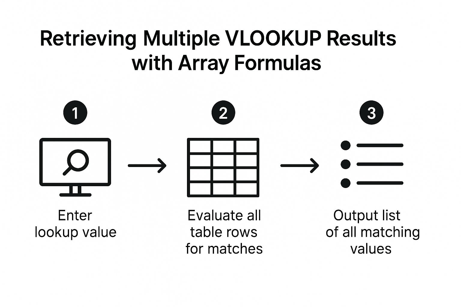
The visualization shows a three-step process: entering the lookup value, evaluating all rows for every match, and finally outputting a dynamic list of all corresponding values, rather than just the first one.

Strategic Breakdown

Imagine you have a list of sales and need to find all products sold by a specific salesperson. A standard VLOOKUP would only return the first product. The array formula to retrieve all products is more complex: =IFERROR(INDEX($B$2:$B$10, SMALL(IF($G$1=$A$2:$A$10, ROW($A$2:$A$10)-ROW($A$1)), ROW(1:1))), ""). Note: This is an array formula and must be entered by pressing Ctrl + Shift + Enter.

• IF($G$1=$A$2:$A$10, ROW($A$2:$A$10)-ROW($A$1)): This core part checks every cell in the salesperson column (A2:A10) for a match with the lookup value (G1). If it finds a match, it returns the relative row number; otherwise, it returns FALSE.
• SMALL(..., ROW(1:1)): The SMALL function takes the array of row numbers and returns the 1st smallest one. As you drag the formula down, ROW(1:1) becomes ROW(2:2), asking for the 2nd smallest row number, and so on.
• INDEX($B$2:$B$10, ...): INDEX then takes this row number and returns the value from the corresponding position in the product column (B2:B10).
• IFERROR(..., ""): This wraps the entire formula to display a blank cell instead of an error once all matches have been listed.

Key Insight: Combining INDEX, SMALL, and an IF statement within an array formula fundamentally changes how Excel looks up data. Instead of a single-value retrieval, you create a dynamic system that can extract and list every single instance of a match, providing a complete view of the data.

Actionable Takeaways

To effectively pull multiple matches, keep these tips in mind:

• Remember Ctrl + Shift + Enter: Array formulas will not work if you just press Enter. You must use the Ctrl + Shift + Enter key combination, which will wrap the formula in curly braces {} in the formula bar.
• Use Helper Columns for Simplicity: If the array formula seems too daunting, you can achieve a similar result by creating a helper column that generates a unique ID for each match (e.g., "John-1", "John-2") and then using a standard VLOOKUP on that new unique ID.
• Transition to FILTER Function: In newer versions of Excel (Microsoft 365), the FILTER function is a much simpler and more efficient alternative. The formula would be =FILTER(B2:B10, A2:A10=G1, "No Matches"), which accomplishes the same goal without the complexity of an array formula.

9 VLOOKUP Formula Use Cases Comparison

Feature / Method	Implementation Complexity 🔄	Resource Requirements ⚡	Expected Outcomes 📊	Ideal Use Cases 💡	Key Advantages ⭐
Basic VLOOKUP with Exact Match	Low 🔄	Low ⚡	Accurate single exact match lookup 📊	Simple lookups needing precise matches 💡	Reliable, easy to implement, consistent ⭐
VLOOKUP with Approximate Match	Medium 🔄	Low ⚡	Closest match less than or equal, range lookups 📊	Graded scales, tax brackets, commissions 💡	Handles missing values smoothly, efficient for sorted data ⭐
VLOOKUP with IFERROR for Error Handling	Medium 🔄	Low ⚡	Custom error messages, cleaner reports 📊	Reports requiring polished output without errors 💡	Prevents formula breaks, improves user experience ⭐
VLOOKUP with Wildcards	Medium 🔄	Medium ⚡	Partial text matching, flexible search 📊	Fuzzy text searches, incomplete data scenarios 💡	Flexible text search, handles variations ⭐
Dynamic VLOOKUP with INDIRECT	High 🔄	Medium ⚡	Dynamic table references based on cell input 📊	Multi-table lookups, dashboards, scenario analysis 💡	Highly flexible and adaptable ⭐
VLOOKUP with CONCATENATE for Multiple Criteria	High 🔄	Medium ⚡	Multi-column criteria lookup, precise matching 📊	Complex lookups with combined criteria 💡	Enables multi-criteria searches, handles duplicates ⭐
VLOOKUP with MATCH for Dynamic Column Selection	High 🔄	Low ⚡	Dynamic column index based on headers 📊	Variable column positions, adaptable table structures 💡	Automatic formula updates, easier maintenance ⭐
VLOOKUP with Array Formulas for Multiple Results	Very High 🔄	High ⚡	Returns multiple matches instead of just first 📊	Detailed reporting, multiple result retrieval 💡	Efficient multiple match handling, comprehensive ⭐

From Formula to Fluency: Your VLOOKUP Mastery Plan

You've just journeyed through a comprehensive collection of VLOOKUP formula examples, moving far beyond basic data retrieval. We've deconstructed everything from the fundamental exact match to sophisticated, dynamic lookups that can adapt to changing data structures. The key takeaway is that VLOOKUP is not just a single tool; it's a foundational component of a much larger data manipulation toolkit within Excel. By understanding its mechanics and its limitations, you unlock the ability to solve complex data challenges with creativity and precision.

The true power of these examples lies not in memorizing syntax, but in internalizing the strategic logic behind each formula. We saw how a simple TRUE argument can transform VLOOKUP into a powerful tool for tiered pricing models, and how IFERROR adds a layer of professional polish by managing user experience and preventing downstream calculation errors. Mastering these nuances is what separates a casual user from a true spreadsheet professional.

Your Strategic Path Forward

To translate this knowledge into practical skill, you need a plan. Don't just file these examples away; actively integrate them into your work. The goal is to move from simply replicating formulas to intuitively constructing them to solve novel problems as they arise.

• Revisit the Fundamentals: Start by solidifying your understanding of TRUE vs. FALSE. This distinction is the most common stumbling block and the source of countless errors. Build a small, sample dataset and practice implementing both approximate and exact matches until their behavior is second nature.
• Embrace Dynamic Solutions: Pay close attention to the examples using MATCH, INDIRECT, and array formulas. These represent a significant leap in capability. The VLOOKUP with MATCH combination, in particular, is a game-changer for creating resilient dashboards and reports that don't break when columns are rearranged.
• Combine and Conquer: The real magic happens when you start nesting VLOOKUP with other functions like CONCATENATE and IFERROR. Practice creating unique lookup keys on the fly and building robust formulas that anticipate and gracefully handle potential errors.

Key Insight: The most advanced Excel users don't just know what a function does; they understand how it interacts with others. Think of VLOOKUP as a verb in a sentence, and functions like MATCH and IFERROR as the adverbs and conjunctions that give it context and power.

Ultimately, mastering these VLOOKUP formula examples is about more than just finding data. It's about building confidence, saving time, and delivering more accurate, insightful, and dynamic reports. It’s about transforming your spreadsheets from static repositories of information into interactive tools that drive better decision-making. Continue to experiment, challenge yourself with new data scenarios, and you will soon find that you are not just using formulas, but thinking in them.

---

Ready to show off your new Excel prowess? As you master complex formulas, embrace the culture with gear that speaks your language. SumproductAddict creates premium apparel and accessories for data professionals who live and breathe spreadsheets. Check out our collection of witty, stylish Excel-themed gear at SumproductAddict and wear your data skills with pride.