Mastering the Excel Depreciation Formula

When you hear "Excel depreciation formula," you might think of a single, scary function. But it's actually a whole suite of them—SLN, DB, DDB, SYD, and VDB—each a powerful tool for calculating how an asset loses value over time.

Learning these isn't just about ticking a box in an accounting course. It's about leveling up your financial game, moving from basic bookkeeping to real strategic planning that impacts everything from tax returns to big investment decisions.

Why Understanding Depreciation in Excel Is a Game Changer

Let's get practical. Calculating depreciation isn't just some chore your accountant handles. It's a core skill for any business that wants a clear financial picture and a strategic edge. When you accurately track how an asset’s value drops over its useful life, it has a direct, tangible effect on your bottom line.

For starters, this process directly shapes your company's tax liability. By recording depreciation as an expense, you lower your reported net income. A lower net income can mean a smaller tax bill. Simple as that.

The real trick is choosing the right method. Whether you go with a steady, predictable formula or an accelerated one can dramatically shift when you get those tax benefits.

Choosing the Right Method for the Right Asset

Think of Excel's depreciation functions as a mechanic's toolbox. You have different tools for different jobs, and you wouldn't use a sledgehammer to tighten a small bolt.

• SLN (Straight-Line): This is your trusty, all-purpose wrench. It spreads the depreciation expense out evenly across every single period of the asset's life. It's perfect for things that lose value at a steady, predictable pace, like office furniture or basic equipment.

• DB (Declining Balance) & DDB (Double Declining Balance): These are your power tools for accelerated depreciation. They front-load the expense, meaning you write off a much larger chunk of the asset's cost in its first few years. This is a fantastic strategy for assets that lose value fast right out of the gate, like company vehicles or new tech hardware.

• SYD (Sum-of-the-Years' Digits): This is another accelerated method, but it's a bit less aggressive than DDB. It's a great middle-ground option, giving you faster depreciation than SLN but a more gradual decline than the DDB method.

• VDB (Variable Declining Balance): Now this is the specialist tool—the most flexible of the bunch. It starts with an accelerated method but can automatically switch over to a straight-line calculation once that becomes more financially beneficial. It's the best of both worlds.

The real power isn't just memorizing the formulas, but knowing when and why to use them. Applying an accelerated method like DDB to a major equipment purchase can deliver immediate tax advantages, freeing up cash flow you can then reinvest in the business.

Ultimately, mastering the Excel depreciation formula is about turning raw numbers into actionable business intelligence. The insights you get from these calculations support smarter capital budgeting, more accurate financial statements, and better asset management overall.

When you feed these calculations into bigger reports, they tell a clear financial story. For instance, you can learn more about how to build a stunning Excel dashboard to visually represent this kind of financial data. This guide will walk you through each function, so you can start applying them with confidence.

Calculating Consistent Value with the SLN Function

When you're first dipping your toes into depreciation, the Straight-Line (SLN) method is the most sensible place to start. It’s the workhorse of depreciation for a good reason—its simplicity and predictability are unmatched, making it a favorite for clean, straightforward financial reporting.

The whole idea behind the SLN function is to spread an asset's cost evenly across its useful life. This consistency is a massive help for financial forecasting because the depreciation expense stays the exact same, year after year. No surprises.

Breaking Down the SLN Formula

Excel's SLN function is refreshingly intuitive. It just needs three key pieces of information (or arguments, in Excel-speak) to do its job.

• Cost: This is simply the initial purchase price of the asset. It’s the full amount you paid to get it up and running.
• Salvage: This is the estimated residual value of the asset when you're done with it. Think of it as the trade-in or resale value you expect to get at the end of its useful life.
• Life: This is the number of periods—usually years—you'll depreciate the asset over. It’s the asset’s expected operational lifespan.

The syntax is as simple as it gets: =SLN(cost, salvage, life). Just plug in those three values, and Excel instantly calculates the depreciation amount for a single period.

A Practical Scenario for SLN

Let's walk through a real-world example. Imagine a small marketing agency buys a new high-end server for $15,000. The IT team figures it will have a useful life of 5 years. After that, they expect to sell it for parts or to a smaller business for a salvage value of $1,500.

To find the annual depreciation, you’d pop this into a cell: =SLN(15000, 1500, 5).

Excel will give you $2,700. This means the agency will record a depreciation expense of $2,700 every single year for five years. It’s a clear, predictable hit to the income statement and a perfect example of using an Excel depreciation formula in practice.

Key Takeaway: The Straight-Line method’s biggest advantage is its simplicity. It gives you a constant, easy-to-track expense that simplifies bookkeeping and long-term financial planning. It’s the perfect fit for assets that lose value consistently over time.

While SLN is fantastic for basic schedules, the real magic happens when you combine its output with other functions for deeper insights. For instance, once you have your annual depreciation figures, you might want to run more complex analyses. To really level up, you should master the SUMPRODUCT function in Excel for multi-conditional summing and unlock more powerful reporting.

Using Accelerated Depreciation with DB and DDB

While the Straight-Line method offers perfect predictability, it doesn’t always reflect reality. Some assets, especially in technology and transportation, lose a huge chunk of their value the moment you put them into service. This is where accelerated depreciation methods become essential.

These methods front-load the depreciation expense, recognizing a larger cost in the early years and less in the later years. From a tax perspective, this can be a powerful strategy, as it often means larger tax deductions sooner rather than later. Excel gives us two fantastic functions for this: DDB (Double Declining Balance) and the more flexible DB (Declining Balance).

The Aggressive Approach with Double Declining Balance (DDB)

The Double Declining Balance (DDB) function is the most common—and aggressive—form of accelerated depreciation. Just as the name implies, it depreciates an asset at twice the rate of the straight-line method. I find myself reaching for it when dealing with assets that become obsolete quickly, like computer hardware or specialized manufacturing equipment.

The syntax for the DDB function is pretty straightforward:

=DDB(cost, salvage, life, period, [factor])

• Cost, Salvage, Life: These are the same arguments you’ll recognize from the SLN function.
• Period: This tells Excel which year of the asset's life you want to calculate depreciation for.
• Factor (Optional): This is where you can tweak the rate. If you leave it blank, Excel defaults to 2, which gives you the "double" in Double Declining Balance.

This aggressive front-loading means your asset's book value drops much faster in the first couple of years, which perfectly mirrors the actual market value loss of many modern assets. To really get a handle on all of Excel's powerful tools, you might find our comprehensive Excel formulas cheat sheet to master key functions easily super helpful.

Getting More Control with the Declining Balance (DB) Function

The Declining Balance (DB) function offers a bit more nuance and control. It also provides accelerated depreciation, but its real advantage is an optional argument that accounts for assets you buy mid-year. This makes it incredibly useful for precise, real-world accounting.

The DB function calculates depreciation by multiplying the asset's book value at the start of a period by a fixed rate. But the secret sauce is its ability to adjust for partial-year depreciation using an optional month parameter, which ensures your calculations are spot-on for assets acquired partway through the year.

The syntax for the DB function is:

=DB(cost, salvage, life, period, [month])

• Month (Optional): This is the number of months in the first year of depreciation. If you omit it, Excel just assumes a full 12 months.

Pro Tip: Use the DB function’s month argument when an asset is purchased late in the fiscal year. This stops you from claiming a full year's depreciation for something you only owned for a few months, keeping your financial statements accurate and compliant.

A Side-by-Side Comparison: DB vs. DDB

Let’s run through a quick scenario. Imagine a tech company buys a new server farm for $250,000. It has a useful life of 5 years and an estimated salvage value of $25,000.

If we use DDB, the depreciation for Year 1 would be =DDB(250000, 25000, 5, 1), which comes out to a hefty $100,000.

But what if the company bought those servers in September, meaning it only owned them for 4 months in the first fiscal year? This is where the DB function truly shines. The formula would be =DB(250000, 25000, 5, 1, 4), resulting in a first-year depreciation of $33,333.

This comparison clearly shows how the DB function gives you a more accurate, prorated excel depreciation formula for partial years, while DDB is your go-to for a simpler, more aggressive write-off when you have the asset for the full year.

Advanced Scenarios with SYD and VDB

Alright, once you've gotten the hang of the basic straight-line and declining balance methods, it's time to level up. Let's dig into two of Excel's more specialized depreciation functions: SYD and VDB.

These aren't your everyday, one-size-fits-all tools. They give you the nuanced control you need for more complex asset management, especially when you need a more tailored approach to accelerated depreciation.

The Balanced Approach of the SYD Function

I often think of the Sum-of-the-Years' Digits (SYD) function as the perfect middle ground. It gives you accelerated depreciation, much like DDB, but the decline isn't nearly as aggressive.

This makes it a fantastic choice when you know an asset loses more value upfront but not at the breakneck pace the double-declining method assumes. It’s a more controlled, less dramatic acceleration.

The function calculates depreciation based on a simple fraction. The denominator is the sum of the digits of the asset's useful life (for a 5-year life, that's 5+4+3+2+1=15), and the numerator is the remaining years of life. This creates a depreciation expense that goes down at a steady rate each year.

The syntax is just as clean: =SYD(cost, salvage, life, per). All the arguments are familiar, with per telling Excel which period you're calculating for.

Let's take our $60,000 asset with a $5,000 salvage value and a 5-year life. Using SYD, the first-year depreciation comes out to $18,333. That's significantly more than the $11,000 from the straight-line method but comfortably less than the $24,000 from DDB. It perfectly illustrates its role as a balanced choice in your Excel depreciation formula toolkit.

The Unmatched Flexibility of the VDB Function

Now, for the real powerhouse. When it comes to complex financial modeling, nothing beats the Variable Declining Balance (VDB) function. This is Excel’s most adaptable depreciation tool by a long shot—a hybrid formula that can handle situations other functions just can't touch.

Its true strength is its ability to calculate depreciation for any period, even partial ones, and its brilliant crossover feature.

VDB can automatically switch from a declining balance method to a straight-line calculation the moment straight-line depreciation becomes greater. This is a game-changer. It ensures the asset is fully depreciated by the end of its life, giving you the best of both worlds: accelerated benefits early on with a clean, precise finish.

The VDB function is your go-to for precision. Its ability to handle partial periods and switch to straight-line calculation makes it invaluable for depreciating assets not purchased at the start of a fiscal year or for building highly accurate, long-term financial forecasts.

Imagine you bought a piece of heavy machinery halfway through the first quarter. With VDB, you can calculate the exact depreciation for that initial partial period and every period after. No guesswork needed.

Here's a quick look at its key arguments:

• start_period: The beginning of the period you want to calculate.
• end_period: The end of that same period.
• factor: The rate for the declining balance (it defaults to 2 for DDB).
• no_switch: This is a simple TRUE/FALSE that tells Excel whether to switch to straight-line. If you set it to FALSE or just leave it blank, it will switch automatically when it makes sense.

This level of control makes VDB the ultimate Excel depreciation formula for those tricky assets with fluctuating usage or for financial models that demand maximum accuracy.

How to Build a Dynamic Depreciation Schedule

Knowing the individual functions is a great start, but the real power comes from combining them into an automated, bullet-proof tool. Let's walk through how to build a dynamic, all-in-one depreciation schedule. The idea is to create a template where you or your team can pick a depreciation method from a simple dropdown and watch the entire schedule update on the fly.

We’re aiming for a reusable worksheet that takes the complex accounting off your plate. It will automatically figure out the opening book value, periodic depreciation, accumulated depreciation, and closing book value for every year of an asset's life.

Setting Up Your Master Template

First things first, let's get the input section of our worksheet structured. Find a clean spot at the top and lay out clear labels for your core asset data. This keeps your variables organized and makes them a breeze to change later on.

You'll want cells for these key inputs:

• Asset Cost: The initial purchase price.
• Salvage Value: What you estimate it's worth at the end of its life.
• Useful Life (Years): The asset's expected operational lifespan.
• Depreciation Method: This will be our interactive dropdown menu.

This kind of setup is foundational for any serious financial modeling. If you want to really go deep on this, we've got a fantastic guide on how to build financial models in Excel from scratch.

Creating a Dropdown for Method Selection

Now for the fun part—making it dynamic. Select the cell right next to your "Depreciation Method" label. Head over to the Data tab on the ribbon, find Data Validation, and in the "Allow" dropdown, choose List.

In the "Source" box that appears, just type in the methods you want to offer, separated by commas: SLN,DDB,SYD. Click OK, and you've got yourself an interactive dropdown. This little menu is about to become the control center for the whole schedule.

Building the Logic with an IF Function

With your inputs ready, it's time to build the actual schedule. Create columns for Year, Opening Book Value, Depreciation Expense, Accumulated Depreciation, and Closing Book Value.

This is where the magic really happens. In your "Depreciation Expense" column, you'll use a nested IF function. This formula will look at the method you selected in the dropdown and then apply the correct Excel depreciation formula.

A basic version of the formula will look something like this: =IF(Method="SLN", SLN(...), IF(Method="DDB", DDB(...), SYD(...)))

You'll just need to fill in the arguments for each function, making sure they point back to your input cells. With one powerful formula, you've created a system that reads your selection and does all the heavy lifting for you.

The infographic below breaks down the logic for the SYD method, showing how it calculates the annual expense using a declining fraction.

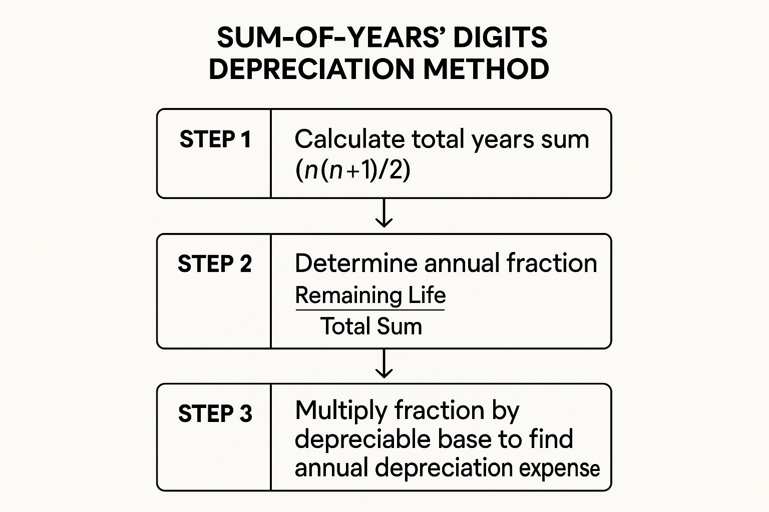
As you can see, the SYD method relies on a systematic reduction in the depreciation fraction each year. This results in a controlled but accelerated write-off early in the asset's life.

With a dynamic schedule like this, you’ve built a sophisticated tool that makes complex depreciation analysis accessible to anyone on your team, no matter their Excel skill level.

Common Questions About Depreciation in Excel

Even after you've got a handle on the functions, you're going to hit some bumps in the road. It happens to everyone. Let's tackle some of the most common questions and sticking points that pop up when you're knee-deep in a depreciation schedule.

A classic scenario is when an asset gets sold before it's fully depreciated. What do you do then? You'll need to figure out the gain or loss on that sale. First, calculate the asset's book value at the exact moment of sale—that’s just the original cost minus all the depreciation you've booked so far. The difference between what you sold it for and that book value is your taxable gain or loss.

Can I Depreciate Land or Intangible Assets?

This is a big one that trips up a lot of people. The short answer for land? A hard no.

Land is considered to have an indefinite useful life, so it's not depreciated. It doesn't wear out or get "used up" like a delivery truck or a computer.

Intangible assets like patents, copyrights, and trademarks are another matter entirely. These are amortized, not depreciated. While the idea is similar—spreading the cost over a set period—the accounting rules and language are different. You won’t use an excel depreciation formula like SLN or DDB for amortization. Instead, you'll most likely set up a simple straight-line calculation manually.

Here's the key takeaway: Depreciation is strictly for tangible assets with a finite, predictable useful life. If you try to apply these functions to land or intangibles, you're going to end up with some seriously inaccurate financial reports.

Troubleshooting Common Formula Errors

What about when Excel screams at you with a #NUM! or #VALUE! error? Don't panic. It's almost always a sign that one of your inputs is off. A #NUM! error in DDB or VDB, for instance, often means your salvage value is higher than the original cost, or you've plugged in a negative number for the asset's life.

Here’s a quick mental checklist:

• Check Your life Argument: Is it a positive whole number representing the total periods?
• Verify salvage Value: It absolutely must be less than the cost.
• Confirm period is Valid: The period you're calculating can't be greater than the asset's total life.

Fixing these is usually a quick correction. If you're still stuck and staring at an error message, there are some great guides out there on how to find and fix errors in Excel that cover more general troubleshooting.

---

Ready to show off your spreadsheet skills in the real world? The apparel and accessories from SumproductAddict are designed for data pros who live and breathe formulas. Grab a witty tee, a formula-packed desk mat, or a custom fleece to celebrate your love for Excel in style. Check out the full collection at https://sumproductaddict.com.