Excel Formulas Cheat Sheet | Master Key Functions Easily

How To Use This Excel Formulas Cheat Sheet

This Excel Formulas Cheat Sheet is your go-to resource for quickly finding and using essential Excel formulas. Whether you're a beginner or an expert, this guide provides a clear and organized way to navigate the world of Excel functions. Each formula is categorized for easy lookup.

This cheat sheet breaks down each formula into three key parts: syntax, purpose, and examples. This consistent structure makes it easy to understand how to apply each formula in practical situations.

Understanding the Formula Structure

Let's say you need to calculate an average. You'd find the AVERAGE function under the "Mathematical and Statistical Functions" category. The entry clearly shows the function's syntax, explaining how to structure the formula correctly. A practical example then demonstrates how the AVERAGE function works in a real-world scenario. This approach applies to every formula listed, ensuring clear and concise guidance. Related formulas and concepts are cross-referenced to enhance your understanding and help you discover useful combinations.

Testing and Implementation

Before using a new formula on a large dataset, test it with a smaller set of data first. This allows you to verify its accuracy and ensure it works as expected. After confirming its functionality, you can then confidently apply it to larger datasets. This careful testing process helps prevent potential errors that could impact important decisions.

With an estimated 0.5 to 1.5 billion users worldwide, Excel plays a vital role in various industries. This widespread usage emphasizes the need for a dependable resource like this cheat sheet. For more in-depth information on Excel's global reach, check out this resource on Excel statistics: Discover more insights.

Mastering Function Parameters

This cheat sheet also helps you understand function parameters. You'll learn to differentiate between required and optional arguments, allowing you to customize formulas for your specific needs. This empowers you to create efficient and dynamic spreadsheets. If you're looking to elevate your data manipulation skills, explore advanced data transformation with Excel Power Query: Check out our guide on: Excel Power Query. Mastering these core Excel concepts will unlock its full potential and boost your spreadsheet proficiency.

Mathematical And Statistical Functions Reference

This Excel formulas cheat sheet covers essential mathematical and statistical functions, helping you transform raw data into meaningful insights. Whether you're performing basic calculations or diving into complex analyses, these functions are the foundation of effective spreadsheet work.

Essential Mathematical Functions

• SUM: The =SUM(number1, [number2], ...) function adds all numbers within a specified range. For example, =SUM(A1:A5) adds the values from cell A1 through A5. This is a fundamental building block for many more complex formulas.

• AVERAGE: Need to calculate the average of a set of numbers? The =AVERAGE(number1, [number2], ...) function is your go-to. =AVERAGE(B1:B10) calculates the average of the values in cells B1 through B10, giving you a quick understanding of central tendencies in your data.

• COUNT: The =COUNT(value1, [value2], ...) function counts the number of cells containing numerical data. For example, =COUNT(C1:C20) counts how many cells within that range contain numbers, helping you understand the size of your numerical datasets.

• PRODUCT: The =PRODUCT(number1, [number2], ...) function multiplies all the given numbers together. =PRODUCT(D1, D2, D3) multiplies the values in D1, D2, and D3. This is particularly useful in financial modeling or scientific calculations.

• ROUND: The =ROUND(number, num_digits) function rounds a number to a specified number of digits. =ROUND(2.345, 2) would round 2.345 to 2.35. This function is essential for managing precision and minimizing rounding errors.

To quickly compare these core functions, refer to the table below:

Core Mathematical Functions Comparison: Quick reference comparing essential mathematical functions with syntax, parameters, and optimal use cases.

Function	Syntax	Primary Purpose	Best Use Case
SUM	=SUM(number1, [number2], ...)	Adds all numbers in a range	Calculating total sales for a month
AVERAGE	=AVERAGE(number1, [number2], ...)	Calculates the average of a set of numbers	Determining the average score on a test
COUNT	=COUNT(value1, [value2], ...)	Counts cells containing numerical data	Finding the number of orders processed
PRODUCT	=PRODUCT(number1, [number2], ...)	Multiplies given numbers together	Calculating compound interest
ROUND	=ROUND(number, num_digits)	Rounds a number to specified digits	Displaying financial data with two decimal places

These functions provide the foundational tools for countless spreadsheet operations.

Key Statistical Functions

Statistical functions go beyond basic math, offering deeper insights into your data. This section of our Excel formulas cheat sheet covers some of the most commonly used ones.

• STDEV: The =STDEV(number1, [number2], ...) function calculates the standard deviation of a dataset, showing how spread out the numbers are. =STDEV(A1:A10) calculates the standard deviation of the values in cells A1 through A10. Understanding standard deviation is key to interpreting data variability.

• MEDIAN: The =MEDIAN(number1, [number2], ...) function finds the middle value in a sorted range. =MEDIAN(B1:B10) returns the median of the numbers in cells B1 through B10. Median is often preferred over average when dealing with datasets potentially skewed by outliers.

• PERCENTILE: Use the =PERCENTILE.INC(array, k) function to return the k-th percentile of values in a range. For example, =PERCENTILE.INC(C1:C100, 0.25) returns the 25th percentile, providing insights into data distribution.

• MIN/MAX: The =MIN(number1, [number2], ...) and =MAX(number1, [number2], ...) functions return the smallest and largest values in a set, respectively. These are useful for quickly identifying the extreme values within your data.

These statistical functions provide a robust toolkit for analyzing data distribution, identifying trends, and drawing meaningful conclusions. This part of the Excel formulas cheat sheet helps you perform more in-depth analysis and make data-driven decisions.

Text Functions For Data Manipulation

This part of our Excel formulas cheat sheet helps you master text manipulation, turning raw text into usable data. Whether you're combining strings or extracting key information, these functions are essential for data cleaning and analysis.

Combining and Extracting Text

• CONCATENATE/TEXTJOIN: Need to combine text from different cells? These are your go-to functions. =CONCATENATE(A1, " ", B1) merges the text in A1 and B1 with a space. =TEXTJOIN(" ", TRUE, A1:A5) joins text from A1 to A5 with a space, conveniently skipping any empty cells.

• LEFT/RIGHT/MID: These functions are perfect for extracting parts of a text string. =LEFT(A1, 3) grabs the first 3 characters from A1. =RIGHT(A1, 4) takes the last 4 characters. =MID(A1, 4, 2) returns 2 characters starting at the 4th position.

Formatting and Cleaning Text

• UPPER/LOWER/PROPER: Keep your text formatting consistent with these functions. =UPPER(A1) transforms text to uppercase. =LOWER(A1) converts it to lowercase. =PROPER(A1) capitalizes the first letter of every word, making titles and names look neat.

For more tips, check out these quick tips for cleaning your data in Excel. They build on these text functions and offer more ways to refine your data skills.

Advanced Text Functions: Finding, Searching, and Replacing

• FIND/SEARCH: These functions locate a specific piece of text within a larger string. =FIND("apple", A1) pinpoints the starting position of "apple" in A1 (case-sensitive). =SEARCH("Apple", A1) does the same, but without case sensitivity.

• SUBSTITUTE/REPLACE: Need to replace text? =SUBSTITUTE(A1, "old", "new") swaps all instances of "old" with "new" in A1. =REPLACE(A1, 5, 3, "new") replaces 3 characters starting at position 5 in A1 with "new," offering more precise control.

Using these advanced text functions alongside the core functions in this Excel formulas cheat sheet equips you to handle nearly any text manipulation task, making your spreadsheets more efficient and dynamic.

Date and Time Functions Mastery Guide

This Excel formulas cheat sheet section covers essential date and time functions. Whether you're managing project timelines, calculating durations, or creating dynamic calendars, understanding these functions is key.

Essential Date and Time Functions

Want to get the current date or date and time? Use =TODAY() for the current date and =NOW() for the current date and time. These functions are dynamic, updating with every spreadsheet recalculation.

Want to create a date value from separate year, month, and day components? Use =DATE(year, month, day). Similarly, create specific times with the =TIME(hour, minute, second) function. These are helpful for building dates from different data sources.

Need to extract specific parts of a date? =YEAR(A1) returns the year of a date in cell A1. =MONTH(A1), =DAY(A1), and =WEEKDAY(A1) extract the month, day, and day of the week, respectively. This allows for precise date analysis and reporting.

Advanced Date and Time Calculations

Often, business calculations require excluding weekends and holidays. The =WORKDAY(start_date, days, [holidays]) function adds workdays to a start date, considering optional holidays. =NETWORKDAYS(start_date, end_date, [holidays]) calculates the working days between two dates.

For accurate duration calculations, use =DATEDIF(start_date, end_date, "unit"). The "unit" defines the output (e.g., "Y" for years, "M" for months, "D" for days). This offers flexibility in duration tracking. For more detailed analysis, check out mastering advanced filters in Excel.

Handling Date Formats and Time Zones

Excel stores dates as numbers, enabling date arithmetic. However, displaying dates in different formats requires understanding number formatting. Custom formats give you precise control. Be aware of time zone differences when using data from multiple locations.

Functions like EDATE (add/subtract months) and EOMONTH (return the last day of the month) offer additional functionality. Convert text to dates using DATEVALUE when dealing with text-based dates. Combining these functions enables you to build dynamic dashboards, track project deadlines, and generate reports.

These date and time functions in our Excel formulas cheat sheet will improve your ability to manage temporal data accurately and build effective spreadsheets.

Logical Functions and Conditional Operations

This Excel formulas cheat sheet focuses on logical functions, giving your spreadsheets the power to make decisions based on your data. These functions are the foundation for building smart and adaptable spreadsheet applications.

The IF Function and Its Variations

The IF function is the core of conditional logic in Excel. It follows this basic syntax: =IF(logical_test, value_if_true, value_if_false).

For example, the formula =IF(A1>10, "Greater than 10", "Less than or equal to 10") checks if the value in cell A1 is greater than 10. It then displays the appropriate message.

You can combine IF statements (nested IF statements) for more complex scenarios. =IF(A1>=90,"A",IF(A1>=80,"B",IF(A1>=70,"C","D"))) sets up a straightforward grading system. This lets you construct intricate decision trees within your spreadsheet.

The IF function works well with AND/OR logic to test multiple conditions. =IF(AND(A1>5,B1<10),"Both True","Not Both True") only returns "Both True" if both conditions are met. Similarly, =IF(OR(A1="Apple",B1="Orange"),"Fruit","Not Fruit") returns "Fruit" if either condition is true. This adds significant flexibility to your formulas.

The IFS Function for Multiple Conditions

For situations with many conditions, the IFS function is a more streamlined option. =IFS(A1>=90,"A",A1>=80,"B",A1>=70,"C",TRUE,"D") accomplishes the same grading system as the nested IF example, but with a cleaner, more readable format. The TRUE at the end acts as a catch-all, ensuring a result is always provided.

Error Handling and Robust Logic

Reliable spreadsheets need good error handling. The IFERROR function handles any error that might occur. =IFERROR(A1/B1,"Error") will display "Error" if dividing A1 by B1 results in an error, such as division by zero. The IFNA function specifically addresses #N/A errors, which are common when using lookup functions.

The SWITCH function gives you another way to evaluate multiple conditions. It's particularly helpful when checking against a single cell's value. =SWITCH(A1,"Apple",1,"Banana",2,"Orange",3,4) assigns a number to each fruit, using 4 as the default if A1 doesn't contain "Apple," "Banana," or "Orange." This function further simplifies your formulas.

By combining these logical functions with others in this Excel formulas cheat sheet, you can build powerful and adaptable spreadsheets. Excel's focus on user-friendliness extends to features like "Analyze Data," which lets you quickly visualize and understand your data, often without needing complex formulas. Learn more about "Analyze Data" here. These features make Excel an effective tool for data analysis and dynamic reporting.

Lookup Functions For Data Retrieval

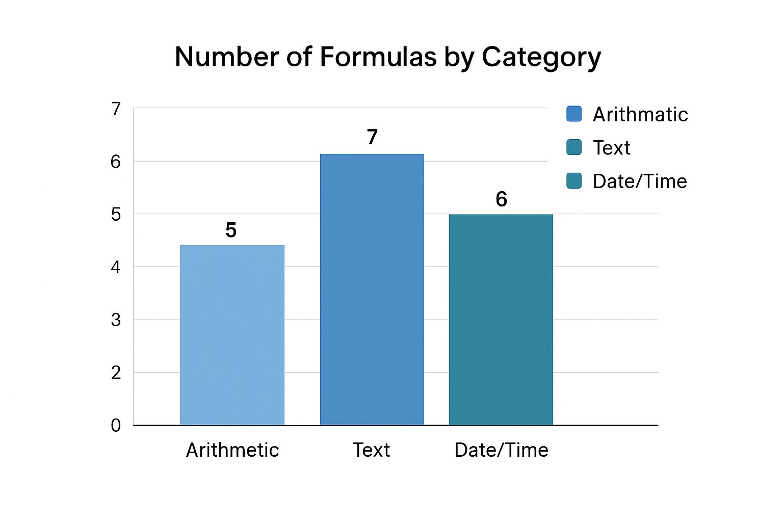
The infographic above categorizes Excel formulas by function: 5 Arithmetic, 7 Text, and 6 Date/Time. Text functions clearly dominate this cheat sheet, emphasizing their importance in data manipulation and cleaning. This section explores lookup functions, essential tools for retrieving specific information from your data.

Mastering VLOOKUP and HLOOKUP

VLOOKUP and HLOOKUP are fundamental functions for vertical and horizontal lookups, respectively. VLOOKUP searches down the first column of a specified range for a given value. If it finds the value, it returns a corresponding value from a designated column in the same row.

For instance, =VLOOKUP(A2, B1:D10, 3, FALSE) searches for the value in cell A2 within the range B1:D10. The FALSE argument ensures an exact match is found. If a match is located, the function returns the value from the third column of the range. HLOOKUP works similarly but searches across rows instead of columns. These functions offer basic lookup capabilities.

Introducing INDEX and MATCH: A Powerful Combination

While VLOOKUP and HLOOKUP are helpful, the combination of INDEX and MATCH provides greater flexibility. INDEX retrieves a value from a specific row and column within a range. MATCH pinpoints the position of a value within a range.

Combining these functions unlocks powerful lookup capabilities. Consider the formula =INDEX(A1:C10, MATCH(D2, B1:B10, 0), 1). MATCH locates the position of the value in D2 within the range B1:B10. INDEX then uses this position to retrieve the corresponding value from the first column of the range A1:C10. This approach allows lookups in any direction, bypassing the column limitations of VLOOKUP.

XLOOKUP: The Next-Generation Lookup Function

XLOOKUP streamlines and improves upon earlier lookup functions with a clearer syntax and enhanced features: =XLOOKUP(lookup_value, lookup_array, return_array, [if_not_found], [match_mode], [search_mode]).

This versatile function handles both exact and approximate matches, searches in either direction, and can even return multiple values. For a comprehensive comparison of XLOOKUP and VLOOKUP, refer to this informative article on the SumproductAddict blog.

Advanced Lookup Techniques

Two-way lookups involve combining INDEX and MATCH twice. This approach allows you to search for a value based on two criteria, such as finding a product price based on both the product name and region.

Dealing with duplicate values requires additional logic, such as using functions like SMALL or LARGE in conjunction with COUNTIF. The INDIRECT function creates dynamic ranges that automatically adjust to changes in your data structure, making your lookup formulas more adaptable.

To help you understand the differences between these powerful functions, take a look at the following table:

Lookup Functions Capability Matrix

Complete comparison of lookup functions showing search direction, flexibility, error handling, and optimal applications.

Function	Search Direction	Flexibility Rating	Error Handling	Optimal Use Case
VLOOKUP	Vertical	Low	#N/A if not found	Simple vertical lookups
HLOOKUP	Horizontal	Low	#N/A if not found	Simple horizontal lookups
INDEX/MATCH	Both	High	Customizable	Complex lookups, two-way lookups
XLOOKUP	Both	Highest	Customizable	Modern replacement for VLOOKUP and HLOOKUP

This table summarizes the key strengths and weaknesses of each lookup function. Notice how XLOOKUP offers the most flexibility and control, while VLOOKUP and HLOOKUP are best suited for simple scenarios. By mastering these functions and techniques, you can efficiently manage and analyze even the largest datasets and create insightful, dynamic reports. This cheat sheet will equip you with the skills to extract information accurately and effectively.

Financial Functions For Business Analysis

This section of our Excel formulas cheat sheet focuses on financial functions, providing the tools you need for smart business decisions and investment analysis. Whether you're calculating loan payments or evaluating project profitability, these functions are essential for anyone working with financial data.

Loan and Investment Calculations

• PV (Present Value): The =PV(rate, nper, pmt, [fv], [type]) function calculates the present value of a loan or investment, helping you determine the current worth of future payments. For example, =PV(0.05/12, 30*12, -1000) calculates the present value of a 30-year mortgage with a 5% annual interest rate and monthly payments of $1,000.

• FV (Future Value): Want to know the future value of your investments? Use the =FV(rate, nper, pmt, [pv], [type]) function. =FV(0.06, 10, -500) shows the future value of investing $500 annually for 10 years at a 6% interest rate.

• PMT (Payment): The =PMT(rate, nper, pv, [fv], [type]) function helps determine the periodic payment for a loan. This is incredibly practical for budgeting and comparing different loan options.

Project Evaluation and Financial Modeling

• NPV (Net Present Value): Evaluate the profitability of a project with =NPV(rate, value1, [value2], ...) which discounts future cash flows to their present value. A positive NPV generally suggests a worthwhile investment.

• IRR (Internal Rate of Return): The =IRR(values, [guess]) function calculates the discount rate that makes the NPV of a project equal to zero. This metric is key for investment analysis and comparing potential projects.

• RATE and NPER: These functions work alongside PV, FV, and PMT to provide a complete picture. RATE calculates the interest rate, and NPER determines the number of periods in a loan or investment, adding detailed financial modeling capabilities to your toolkit. For a deeper dive into building financial models with these functions, check out this guide on how to build these in Excel. Microsoft is well-known for developing versatile tools like Excel and Power Query.

Advanced Financial Functions and Depreciation

• XNPV and XIRR: These functions handle irregular cash flows, providing more accurate calculations for complex investments which is essential for advanced financial modeling.

• Depreciation Functions: Excel offers functions like DB (declining balance), DDB (double-declining balance), and SLN (straight-line) to calculate asset depreciation, vital for accounting and financial reporting. These cater to different depreciation methods.

While precise user statistics for Excel independent of the Microsoft Office suite are difficult to find, past reports indicate a vast user base. In 2015, Microsoft reported 1.1 billion users for their productivity services, including Office. Find more details here. This demonstrates Excel's widespread use across various industries.

These financial functions make Excel a powerful tool for business analysis, empowering you to make informed decisions based on solid financial data.

Want to show off your Excel skills? Visit SumproductAddict for unique Excel-themed apparel and accessories. From t-shirts to desk mats, you'll find something to celebrate your spreadsheet passion.